mf6adj demonstration using the synthetic dewatering example
In this notebook, we show how mf6adj can be used with a MODFLOW 6 version of the synthetic mine dewatering example presented by White et al. (2025), “Reliable Trade-offs Between Environment and Economy: Implications for Mine Dewatering and Managed Aquifer Recharge.”
Import Packages
[1]:
import os
import pathlib as pl
import platform
import shutil
import sys
from datetime import datetime

import flopy
import h5py
import matplotlib.pyplot as plt
import numpy as np
import pandas as pd
import pyemu
[2]:
try:
    import mf6adj
except ImportError:
    sys.path.insert(0, str(pl.Path("../").resolve()))
    import mf6adj
[3]:
mf6_bin, lib_name = mf6adj.get_conda_mf6_paths()
print(f"Using MF6 binary: {mf6_bin}")
print(f"Using MF6 library: {lib_name}")
Using MF6 binary: /home/runner/work/mf6adj/mf6adj/.pixi/envs/default/bin/mf6
Using MF6 library: /home/runner/work/mf6adj/mf6adj/.pixi/envs/default/bin/libmf6.so
Now let’s get the model files we will use. They are stored in the autotest directory.
Copy the MODFLOW Model
[4]:
org_ws = pl.Path("synthdewater")
assert pl.Path(org_ws).exists()
Set up a local copy of the model files.
[5]:
ws = pl.Path("synthdewater_working")
if pl.Path(ws).exists():
    shutil.rmtree(ws)
shutil.copytree(org_ws, ws)
[5]:
PosixPath('synthdewater_working')
[6]:
sim = flopy.mf6.MFSimulation.load(sim_ws=ws)
m = sim.get_model()
X, Y = m.modelgrid.xcellcenters, m.modelgrid.ycellcenters
loading simulation...
  loading simulation name file...
  loading tdis package...
  loading model gwf6...
    loading package dis...
    loading package npf...
    loading package sto...
    loading package ic...
    loading package oc...
    loading package drn...
    loading package rch...
    loading package ghb...
    loading package wel...
    loading package wel...
    loading package obs...
  loading solution package model...
[7]:
def plot_model(k, arr, units=None, cmap="plasma", center=False, levels=None):
    vmin = None
    vmax = None

    if center:
        mx = np.nanmax(np.abs(arr))
        vmin = -1.0 * mx
        vmax = mx
        cmap = "coolwarm"

    fig, ax = plt.subplots(1, 1, figsize=(6, 6))
    ax.set_aspect("equal")
    mv = flopy.plot.PlotMapView(model=m, ax=ax)
    mv.plot_bc("WEL-dewater", label="Dewater Wells")
    mv.plot_bc("WEL-mar", label="Injection Wells")

    mv.plot_bc("DRN", color="green", label="Drain - GDE")
    mv.plot_bc("GHB", color="blue", label="GHB - regional aquifer")
    cb = ax.pcolormesh(X, Y, arr, cmap=cmap, vmin=vmin, vmax=vmax, alpha=0.5)

    plt.colorbar(cb, ax=ax, label=units)
    if levels is not None:
        c = "w"
        if center:
            c = "k"
        CS = ax.contour(X, Y, arr, levels=levels, colors=c)
        ax.clabel(CS, CS.levels, fontsize=10)

    return fig, ax
[8]:
fig, ax = plot_model(0, m.dis.idomain.array[0, :, :].astype(float))
_ = ax.set_title("idomain")
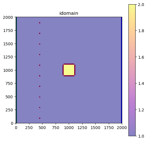
The pit is located in the idomain == 2 region.
[9]:
fig, ax = plt.subplots()
mv = flopy.plot.PlotMapView(model=m)
mv.plot_grid(lw=0.5)
mv.plot_bc("WEL-dewater", label="Dewater Wells")
mv.plot_bc("WEL-mar", label="Injection Wells")

mv.plot_bc("DRN", color="green", label="Drain - GDE")
mv.plot_bc("GHB", color="blue", label="GHB - regional aquifer")

# mv.plot_array(gwf.dis.idomain.get_data(), color='gray', alpha=1)
[9]:
<matplotlib.collections.QuadMesh at 0x7fce50fed690>
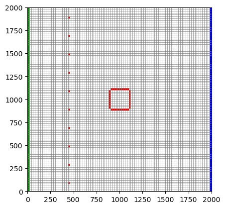
Here we see the GDE DRN boundary on the left, the inflow GHB on the right, and the dewatering and reinjection wells. The model has three stress periods: pre-development (steady state), active mining (10-year transient), and closure (20-year transient).
[10]:
fig, ax = plot_model(0, np.log10(m.npf.k.array[0, :, :]), levels=3)
_ = ax.set_title("HK")
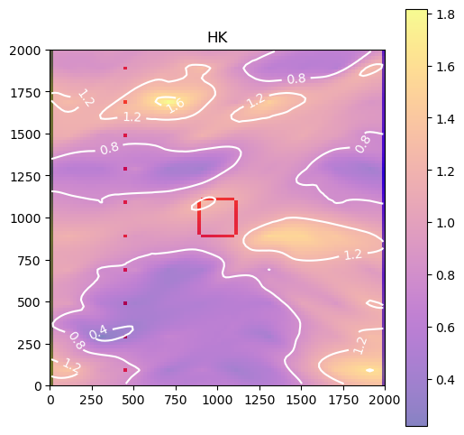
A beautiful example of nonstationary geostatistics.
Run the existing model in our local workspace.
[11]:
pyemu.os_utils.run(mf6_bin.name, cwd=ws)
mf6
                                   MODFLOW 6
                U.S. GEOLOGICAL SURVEY MODULAR HYDROLOGIC MODEL
                        VERSION 6.8.0.dev0+a6a4984.dirty
                               ***DEVELOP MODE***

   MODFLOW 6 compiled Jun 01 2026 18:46:14 with Intel(R) Fortran Intel(R) 64
   Compiler Classic for applications running on Intel(R) 64, Version 2021.6.0
                             Build 20220226_000000

This software is preliminary or provisional and is subject to
revision. It is being provided to meet the need for timely best
science. The software has not received final approval by the U.S.
Geological Survey (USGS). No warranty, expressed or implied, is made
by the USGS or the U.S. Government as to the functionality of the
software and related material nor shall the fact of release
constitute any such warranty. The software is provided on the
condition that neither the USGS nor the U.S. Government shall be held
liable for any damages resulting from the authorized or unauthorized
use of the software.


 MODFLOW runs in SEQUENTIAL mode

 Run start date and time (yyyy/mm/dd hh:mm:ss): 2026/06/02 18:34:43

 Writing simulation list file: mfsim.lst
 Using Simulation name file: mfsim.nam

    Solving:  Stress period:     1    Time step:     1
    Solving:  Stress period:     2    Time step:     1
    Solving:  Stress period:     3    Time step:     1

 Run end date and time (yyyy/mm/dd hh:mm:ss): 2026/06/02 18:34:44
 Elapsed run time:  0.924 Seconds

 Normal termination of simulation.
Now plot some heads.
[12]:
labels = ["predev", "end of mining", "closure"]
hds = flopy.utils.HeadFile(pl.Path(ws) / "model.hds")
for kper, label in enumerate(labels):
    final_arr = hds.get_data(kstpkper=(0, kper))
    fig, ax = plot_model(0, final_arr[0, :, :], units="meters", levels=5)
    ax.set_title(label)
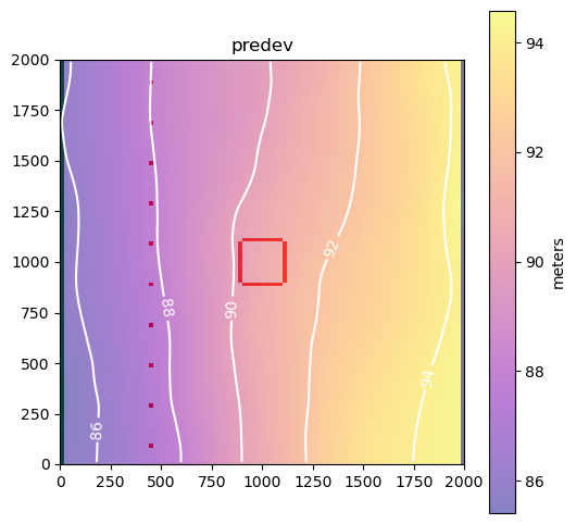
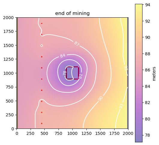
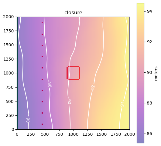
As expected, groundwater flows from high head to low head.
The main requirement for using mf6adj is an input file that describes the performance measures. Fortunately, this file follows a modern format similar to other MF6 input files. Here we will build these measures programmatically so we can examine the pit head at the end of mining and the GDE-boundary flux during pre-development, end-of-mining, and post-closure conditions.
[13]:
drn = pd.DataFrame.from_records(m.drn.stress_period_data.array[0])
drn
[13]:
| cellid | elev | cond | boundname | |
|---|---|---|---|---|
| 0 | (0, 0, 0) | 85 | 100 | drn-gde |
| 1 | (0, 1, 0) | 85 | 100 | drn-gde |
| 2 | (0, 2, 0) | 85 | 100 | drn-gde |
| 3 | (0, 3, 0) | 85 | 100 | drn-gde |
| 4 | (0, 4, 0) | 85 | 100 | drn-gde |
| ... | ... | ... | ... | ... |
| 95 | (0, 95, 0) | 85 | 100 | drn-gde |
| 96 | (0, 96, 0) | 85 | 100 | drn-gde |
| 97 | (0, 97, 0) | 85 | 100 | drn-gde |
| 98 | (0, 98, 0) | 85 | 100 | drn-gde |
| 99 | (0, 99, 0) | 85 | 100 | drn-gde |
100 rows × 4 columns
[14]:
names = ["drn-gde-predev", "drn-gde-endmining", "drn-gde-postclosure"]
pm_fname = "prefmeas.dat"
fpm = open(pl.Path(ws) / pm_fname, "w")

for kper, name in enumerate(names):
    fpm.write(f"begin performance_measure {name}\n")

    for kij in drn.cellid.values:
        fpm.write(
            f"{kper + 1} 1 {kij[0] + 1} {kij[1] + 1} {kij[2] + 1} "
            + "drn-gde direct 1.0 -1.0e+30\n"
        )
    fpm.write("end performance_measure\n\n")
[15]:
name = "pithead-endmining"

kij = (0, 49, 49)
fpm.write(f"begin performance_measure {name}\n")
fpm.write(
    f"{kper + 1} 1 {kij[0] + 1} {kij[1] + 1} {kij[2] + 1} head direct 1.0 -1.0e+30\n"
)
fpm.write("end performance_measure\n\n")
fpm.close()
Run mf6adj
Now we should be ready to go. The adjoint solution process requires one forward model run and then a solve for the adjoint state, which uses the forward solution components (for example, the conductance matrix, RHS, heads, and saturation). The adjoint solve has two important characteristics: it is linear, regardless of the forward model’s linearity, and it proceeds backward in time, starting with the last stress period.
The adjoint solve is slower than the forward run because most of the time is spent in the NumPy sparse linear solve.
[16]:
forward_hdf5_name = "forward.hdf5"
start = datetime.now()

adj = mf6adj.Mf6Adj(
    pm_fname,
    lib_name,
    logging_level="INFO",
    working_directory=ws,
)
adj.solve_forward_model(
    hdf5_name=forward_hdf5_name
)  # solve the standard forward solution
dfsum = adj.solve_adjoint()  # solve the adjoint state for each performance measure
adj.finalize()  # release components
duration = (datetime.now() - start).total_seconds()
print("took:", duration)
2026-06-02 18:34:45,028 - Logger instance 'Mf6Adj-prefmeas-08898fe3' created.
2026-06-02 18:34:45,028 - Running from /home/runner/work/mf6adj/mf6adj/examples/synthdewater_working
2026-06-02 18:34:45,029 - Structured grid found
2026-06-02 18:34:45,075 - MODFLOW 6 version: 6.8.0.dev0
2026-06-02 18:34:45,076 - Processing adjoint file: prefmeas.dat
2026-06-02 18:34:45,081 - Starting flow solution
2026-06-02 18:34:45,297 - Flow (stress period,time step) (1,1) converged in 10 iters, took  0.0035582 mins
2026-06-02 18:34:45,423 - Flow (stress period,time step) (2,1) converged in 5 iters, took   0.001882 mins
2026-06-02 18:34:45,965 - Flow (stress period,time step) (3,1) converged in 25 iters, took  0.0088393 mins
2026-06-02 18:34:45,977 - Flow solution finished and took   0.014921 minutes
2026-06-02 18:34:45,987 - Starting solve_adjoint at 2026-06-02 18:34:45.987880
2026-06-02 18:34:45,991 - Structured grid found, shape: (1, 100, 100)
2026-06-02 18:34:45,994 - Starting adjoint solve for PerfMeas: drn-gde-predev (kper, kstp) (3, 1)
2026-06-02 18:34:45,997 - Solving for lambda
2026-06-02 18:34:45,998 - Solving with direct with solver options: {'use_umfpack': True}
2026-06-02 18:34:46,027 - Solving for lambda took: 0.030207 seconds
2026-06-02 18:34:46,177 - Adjoint solve took: 0.183344 seconds to solve adjoint solution for PerfMeas: drn-gde-predev (kper, kstp) (3, 1)
2026-06-02 18:34:46,178 - Write group to hdf file
2026-06-02 18:34:46,209 - Starting adjoint solve for PerfMeas: drn-gde-predev (kper, kstp) (2, 1)
2026-06-02 18:34:46,212 - Solving for lambda
2026-06-02 18:34:46,212 - Solving with direct with solver options: {'use_umfpack': True}
2026-06-02 18:34:46,241 - Solving for lambda took: 0.0288 seconds
2026-06-02 18:34:46,385 - Adjoint solve took: 0.176107 seconds to solve adjoint solution for PerfMeas: drn-gde-predev (kper, kstp) (2, 1)
2026-06-02 18:34:46,386 - Write group to hdf file
2026-06-02 18:34:46,416 - Starting adjoint solve for PerfMeas: drn-gde-predev (kper, kstp) (1, 1)
2026-06-02 18:34:46,419 - Solving for lambda
2026-06-02 18:34:46,419 - Solving with direct with solver options: {'use_umfpack': True}
2026-06-02 18:34:46,448 - Solving for lambda took: 0.029655 seconds
2026-06-02 18:34:46,591 - Adjoint solve took: 0.17554 seconds to solve adjoint solution for PerfMeas: drn-gde-predev (kper, kstp) (1, 1)
2026-06-02 18:34:46,592 - Write group to hdf file
2026-06-02 18:34:46,619 - Formulate composite sensitivities
2026-06-02 18:34:46,620 - Writing composite sensitivities
2026-06-02 18:34:46,645 - Adjoint solve took:    0.65713 seconds for pm 'drn-gde-predev' at (kper,kstp) (1, 1)
2026-06-02 18:34:46,645 - Starting solve_adjoint at 2026-06-02 18:34:46.645806
2026-06-02 18:34:46,649 - Structured grid found, shape: (1, 100, 100)
2026-06-02 18:34:46,652 - Starting adjoint solve for PerfMeas: drn-gde-endmining (kper, kstp) (3, 1)
2026-06-02 18:34:46,654 - Solving for lambda
2026-06-02 18:34:46,655 - Solving with direct with solver options: {'use_umfpack': True}
2026-06-02 18:34:46,684 - Solving for lambda took: 0.029558 seconds
2026-06-02 18:34:46,830 - Adjoint solve took: 0.178182 seconds to solve adjoint solution for PerfMeas: drn-gde-endmining (kper, kstp) (3, 1)
2026-06-02 18:34:46,831 - Write group to hdf file
2026-06-02 18:34:46,860 - Starting adjoint solve for PerfMeas: drn-gde-endmining (kper, kstp) (2, 1)
2026-06-02 18:34:46,863 - Solving for lambda
2026-06-02 18:34:46,864 - Solving with direct with solver options: {'use_umfpack': True}
2026-06-02 18:34:46,893 - Solving for lambda took: 0.029799 seconds
2026-06-02 18:34:47,039 - Adjoint solve took: 0.178967 seconds to solve adjoint solution for PerfMeas: drn-gde-endmining (kper, kstp) (2, 1)
2026-06-02 18:34:47,040 - Write group to hdf file
2026-06-02 18:34:47,070 - Starting adjoint solve for PerfMeas: drn-gde-endmining (kper, kstp) (1, 1)
2026-06-02 18:34:47,072 - Solving for lambda
2026-06-02 18:34:47,073 - Solving with direct with solver options: {'use_umfpack': True}
2026-06-02 18:34:47,101 - Solving for lambda took: 0.028632 seconds
2026-06-02 18:34:47,246 - Adjoint solve took: 0.175937 seconds to solve adjoint solution for PerfMeas: drn-gde-endmining (kper, kstp) (1, 1)
2026-06-02 18:34:47,247 - Write group to hdf file
2026-06-02 18:34:47,275 - Formulate composite sensitivities
2026-06-02 18:34:47,275 - Writing composite sensitivities
2026-06-02 18:34:47,299 - Adjoint solve took:    0.65372 seconds for pm 'drn-gde-endmining' at (kper,kstp) (1, 1)
2026-06-02 18:34:47,300 - Starting solve_adjoint at 2026-06-02 18:34:47.300422
2026-06-02 18:34:47,304 - Structured grid found, shape: (1, 100, 100)
2026-06-02 18:34:47,306 - Starting adjoint solve for PerfMeas: drn-gde-postclosure (kper, kstp) (3, 1)
2026-06-02 18:34:47,309 - Solving for lambda
2026-06-02 18:34:47,309 - Solving with direct with solver options: {'use_umfpack': True}
2026-06-02 18:34:47,337 - Solving for lambda took: 0.028169 seconds
2026-06-02 18:34:47,483 - Adjoint solve took: 0.176592 seconds to solve adjoint solution for PerfMeas: drn-gde-postclosure (kper, kstp) (3, 1)
2026-06-02 18:34:47,483 - Write group to hdf file
2026-06-02 18:34:47,513 - Starting adjoint solve for PerfMeas: drn-gde-postclosure (kper, kstp) (2, 1)
2026-06-02 18:34:47,515 - Solving for lambda
2026-06-02 18:34:47,516 - Solving with direct with solver options: {'use_umfpack': True}
2026-06-02 18:34:47,545 - Solving for lambda took: 0.029788 seconds
2026-06-02 18:34:47,686 - Adjoint solve took: 0.173744 seconds to solve adjoint solution for PerfMeas: drn-gde-postclosure (kper, kstp) (2, 1)
2026-06-02 18:34:47,687 - Write group to hdf file
2026-06-02 18:34:47,716 - Starting adjoint solve for PerfMeas: drn-gde-postclosure (kper, kstp) (1, 1)
2026-06-02 18:34:47,719 - Solving for lambda
2026-06-02 18:34:47,719 - Solving with direct with solver options: {'use_umfpack': True}
2026-06-02 18:34:47,748 - Solving for lambda took: 0.029126 seconds
2026-06-02 18:34:47,894 - Adjoint solve took: 0.177983 seconds to solve adjoint solution for PerfMeas: drn-gde-postclosure (kper, kstp) (1, 1)
2026-06-02 18:34:47,895 - Write group to hdf file
2026-06-02 18:34:47,923 - Formulate composite sensitivities
2026-06-02 18:34:47,924 - Writing composite sensitivities
2026-06-02 18:34:47,947 - Adjoint solve took:    0.64718 seconds for pm 'drn-gde-postclosure' at (kper,kstp) (1, 1)
2026-06-02 18:34:47,948 - Starting solve_adjoint at 2026-06-02 18:34:47.948327
2026-06-02 18:34:47,952 - Structured grid found, shape: (1, 100, 100)
2026-06-02 18:34:47,954 - Starting adjoint solve for PerfMeas: pithead-endmining (kper, kstp) (3, 1)
2026-06-02 18:34:47,956 - Solving for lambda
2026-06-02 18:34:47,956 - Solving with direct with solver options: {'use_umfpack': True}
2026-06-02 18:34:47,986 - Solving for lambda took: 0.029772 seconds
2026-06-02 18:34:48,135 - Adjoint solve took: 0.181327 seconds to solve adjoint solution for PerfMeas: pithead-endmining (kper, kstp) (3, 1)
2026-06-02 18:34:48,136 - Write group to hdf file
2026-06-02 18:34:48,166 - Starting adjoint solve for PerfMeas: pithead-endmining (kper, kstp) (2, 1)
2026-06-02 18:34:48,168 - Solving for lambda
2026-06-02 18:34:48,169 - Solving with direct with solver options: {'use_umfpack': True}
2026-06-02 18:34:48,198 - Solving for lambda took: 0.029929 seconds
2026-06-02 18:34:48,360 - Adjoint solve took: 0.194032 seconds to solve adjoint solution for PerfMeas: pithead-endmining (kper, kstp) (2, 1)
2026-06-02 18:34:48,361 - Write group to hdf file
2026-06-02 18:34:48,390 - Starting adjoint solve for PerfMeas: pithead-endmining (kper, kstp) (1, 1)
2026-06-02 18:34:48,392 - Solving for lambda
2026-06-02 18:34:48,393 - Solving with direct with solver options: {'use_umfpack': True}
2026-06-02 18:34:48,422 - Solving for lambda took: 0.029311 seconds
2026-06-02 18:34:48,569 - Adjoint solve took: 0.178553 seconds to solve adjoint solution for PerfMeas: pithead-endmining (kper, kstp) (1, 1)
2026-06-02 18:34:48,569 - Write group to hdf file
2026-06-02 18:34:48,597 - Formulate composite sensitivities
2026-06-02 18:34:48,598 - Writing composite sensitivities
2026-06-02 18:34:48,622 - Adjoint solve took:    0.67405 seconds for pm 'pithead-endmining' at (kper,kstp) (1, 1)
2026-06-02 18:34:48,623 - Finalizing Mf6Adj
took: 3.628568
Plot the Results
Done. Let’s see what happened.
[17]:
hdf5_files = [f for f in os.listdir(ws) if f.endswith("hdf5")]
hdf5_files.sort()
hdf5_files = hdf5_files[:-1]
hdf5_files
[17]:
['adjoint_solution_drn-gde-endmining.hdf5',
 'adjoint_solution_drn-gde-postclosure.hdf5',
 'adjoint_solution_drn-gde-predev.hdf5',
 'adjoint_solution_pithead-endmining.hdf5']
mf6adj uses the widely available HDF5 format to store information. These files hold low-level details about the adjoint solution. However, mf6adj.solve_adjoint() also returns a higher-level summary of the results. Let’s look at that first:
[18]:
type(dfsum)
[18]:
dict
[19]:
list(dfsum.keys())
[19]:
['drn-gde-predev',
 'drn-gde-endmining',
 'drn-gde-postclosure',
 'pithead-endmining']
[20]:
dfhw = dfsum["pithead-endmining"]
dfhw
[20]:
| k11 | k33 | wel6_q | rch6_recharge | drn-gde_elev | drn-gde_cond | ghb-inflow_bhead | ghb-inflow_cond | ss | |
|---|---|---|---|---|---|---|---|---|---|
| node | |||||||||
| 1 | -0.000038 | 0.0 | 0.000063 | 0.000063 | 0.0 | -0.005405 | 0.0 | 0.000000 | 0.000052 |
| 2 | -0.000077 | 0.0 | 0.000073 | 0.000073 | 0.0 | 0.000000 | 0.0 | 0.000000 | 0.000069 |
| 3 | -0.000075 | 0.0 | 0.000082 | 0.000082 | 0.0 | 0.000000 | 0.0 | 0.000000 | 0.000087 |
| 4 | -0.000073 | 0.0 | 0.000091 | 0.000091 | 0.0 | 0.000000 | 0.0 | 0.000000 | 0.000108 |
| 5 | -0.000072 | 0.0 | 0.000100 | 0.000100 | 0.0 | 0.000000 | 0.0 | 0.000000 | 0.000131 |
| ... | ... | ... | ... | ... | ... | ... | ... | ... | ... |
| 9996 | 0.000012 | 0.0 | 0.000102 | 0.000102 | 0.0 | 0.000000 | 0.0 | 0.000000 | 0.000323 |
| 9997 | 0.000012 | 0.0 | 0.000099 | 0.000099 | 0.0 | 0.000000 | 0.0 | 0.000000 | 0.000303 |
| 9998 | 0.000012 | 0.0 | 0.000096 | 0.000096 | 0.0 | 0.000000 | 0.0 | 0.000000 | 0.000283 |
| 9999 | 0.000014 | 0.0 | 0.000092 | 0.000092 | 0.0 | 0.000000 | 0.0 | 0.000000 | 0.000263 |
| 10000 | 0.000007 | 0.0 | 0.000089 | 0.000089 | 0.0 | 0.000000 | 0.0 | -0.008336 | 0.000243 |
10000 rows × 9 columns
Those are the node-scale sensitivities for the end-of-mining pit groundwater-level performance measure. Plotting them is easiest using the HDF5 file itself.
[21]:
result_hdf = hdf5_files[-1]
hdf = h5py.File(pl.Path(ws) / result_hdf, "r")
keys = list(hdf.keys())
keys.sort()
print(keys)
['composite', 'solution_kper:00000_kstp:00000', 'solution_kper:00001_kstp:00000', 'solution_kper:00002_kstp:00000']
The composite group contains sensitivities of the performance measure to the model inputs, summed across all adjoint solutions.
[22]:
grp = hdf["composite"]
plot_keys = [
    i for i in grp.keys() if len(grp[i].shape) == 3 and ("k11" in i or "ss" in i)
]
plot_keys
[22]:
['k11', 'ss']
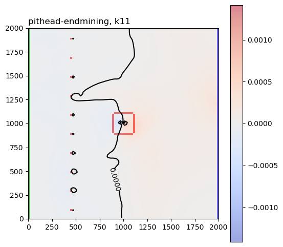
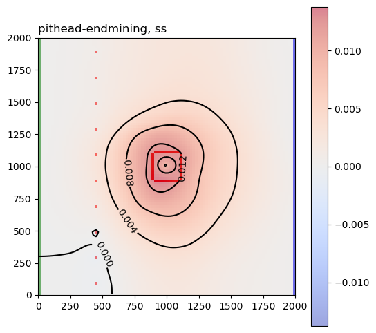
Here is a simple routine to plot these sensitivities.
[23]:
for pkey in plot_keys:
    arr = grp[pkey][:]
    for k, karr in enumerate(arr):
        karr[karr == 0.0] = np.nan
        fig, ax = plot_model(k, karr, center=True, levels=4)
        ax.set_title(pkey + f", layer:{k + 1}", loc="left")
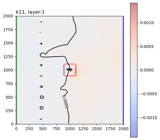
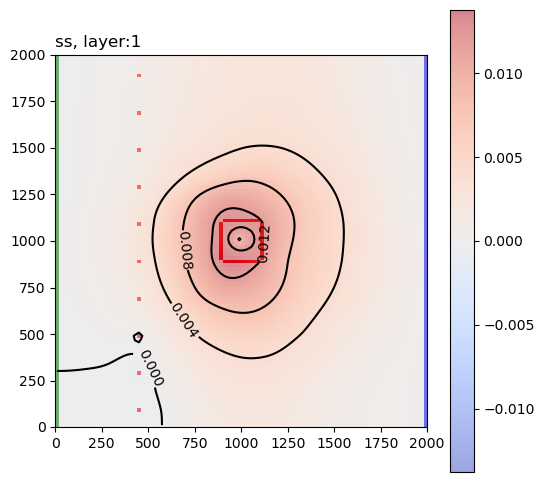
These are the sensitivity maps for end-of-mining pit groundwater level with respect to hk and ss. Are these patterns what you expected?
Now let’s look at the same plots for the GDE-flux performance measures:
[24]:
for result_hdf in hdf5_files:
    hdf = h5py.File(pl.Path(ws) / result_hdf, "r")
    grp = hdf["composite"]
    pm_name = (
        result_hdf.replace("adjoint_solution_", "")
        .split(".")[0]
        .replace("_forward", "")
    )
    for pkey in plot_keys:
        arr = grp[pkey][:]
        for k, karr in enumerate(arr):
            karr[karr == 0.0] = np.nan
            fig, ax = plot_model(k, karr, center=True, levels=4)
            ax.set_title(pm_name + ", " + pkey, loc="left")
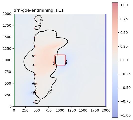
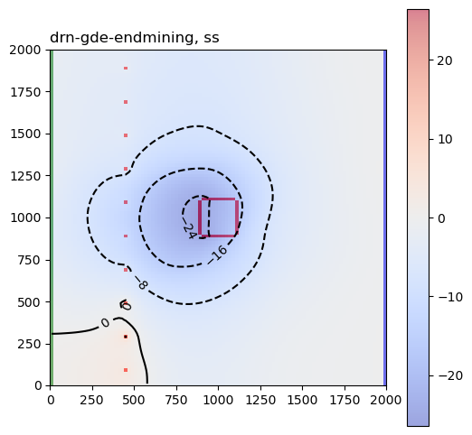
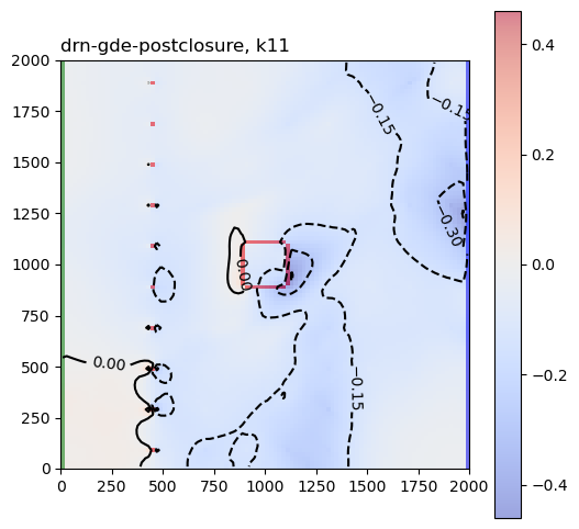
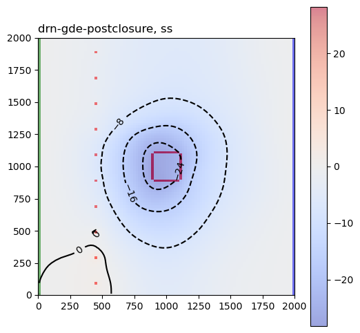
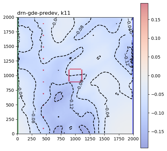
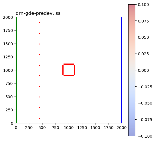
Are those sensitivities consistent with your expectations and hydrologic intuition? Let’s look at the hk array again:
[25]:
fig, ax = plot_model(0, np.log10(m.npf.k.array[0, :, :]), levels=3)
_ = ax.set_title("HK")

Let’s also look at the sensitivity of groundwater pumping during the active mining period to the head in the pit at the end of mining:
[26]:
keys
[26]:
['composite',
 'solution_kper:00000_kstp:00000',
 'solution_kper:00001_kstp:00000',
 'solution_kper:00002_kstp:00000']
[27]:
mining_grp = [key for key in keys if key.startswith("solution_kper:00001")]
assert len(mining_grp) == 1
mining_grp = mining_grp[0]
mining_grp
[27]:
'solution_kper:00001_kstp:00000'
[28]:
plot_keys = [i for i in grp.keys() if len(grp[i].shape) == 3 and ("wel6_q" in i)]
plot_keys
[28]:
['wel6_q']
[29]:
for result_hdf in hdf5_files:
    hdf = h5py.File(pl.Path(ws) / result_hdf, "r")
    grp = hdf[mining_grp]
    pm_name = (
        result_hdf.replace("adjoint_solution_", "")
        .split(".")[0]
        .replace("_forward", "")
    )
    for pkey in plot_keys:
        arr = grp[pkey][:]
        for k, karr in enumerate(arr):
            karr[karr == 0.0] = np.nan
            fig, ax = plot_model(k, karr, center=True, levels=4)
            ax.set_title(pm_name + ", " + pkey, loc="left")
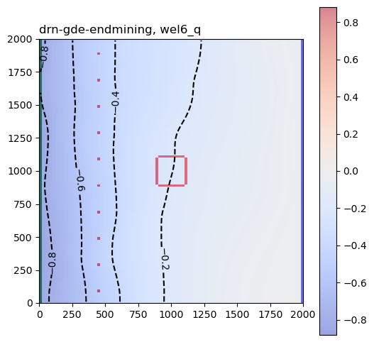
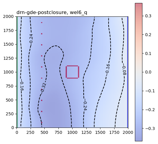
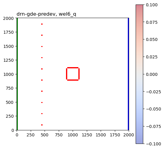
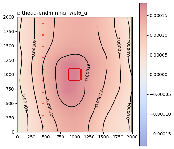
This helps show how groundwater extraction and reinjection during active mining influence both pit groundwater levels and GDE flux at the end of mining and at the end of the closure period.
[ ]:
[ ]: