mf6adj demonstration using the Zaidel water table problem

This problem uses the Zaidel (2003) problem to test the adjoint tool. The Zaidel problem is often used to verify the numerical stability and convergence of a computer code against a discontinuous, steady-state analytical solution of the Boussinesq equation. Here, we use it as a vehicle for understanding the utility of mf6adj.

The learning objectives are:

1. Build and solve the adjoint system for the Zaidel problem using a direct-head performance measure (PM).

2. Understand the adjoint sensitivity results.

3. Explore how the adjoint sensitivity results change for a different PM location.

Import Packages

import os
import pathlib as pl
import platform
import shutil
import sys
from datetime import datetime

import flopy
import h5py
import matplotlib.pyplot as plt
import numpy as np
import pyemu

try:
    import mf6adj
except ImportError:
    sys.path.insert(0, str(pl.Path("../").resolve()))
    import mf6adj

mf6_bin, lib_name = mf6adj.get_conda_mf6_paths()
print(f"Using MF6 binary: {mf6_bin}")
print(f"Using MF6 library: {lib_name}")

Using MF6 binary: /home/runner/work/mf6adj/mf6adj/.pixi/envs/default/bin/mf6
Using MF6 library: /home/runner/work/mf6adj/mf6adj/.pixi/envs/default/bin/libmf6.so

sim_name = "ex-gwf-zaidel"
workspace = pl.Path(sim_name)
if pl.Path(workspace).exists():
    shutil.rmtree(workspace)
pl.Path(workspace).mkdir()

The Zaidel model comprises a steady-state, single-stress-period, single-timestep, two-dimensional stair-stepped domain with a constant-head boundary condition (BC) at both ends controlling the head gradient. No other BCs are applied. At the time this notebook was developed (October 2024), mf6adj was not yet able to handle CHD boundaries directly, so we use the standard workaround of representing a CHD with a general-head boundary that has a high conductance.

We will wrap the model build and run calls in a function so we can test a few additional cases later in the example.

Build the MODFLOW Model

# Model parameters
nper = 1  # Number of periods
nlay = 1  # Number of layers
nrow = 1  # Number of rows
ncol = 200  # Number of columns
delr = 5.0  # Column width ($m$)
delc = 1.0  # Row width ($m$)
top = 25.0  # Top of the model ($m$)
strt = 23.0  # Starting head ($m$)
icelltype = 1  # Cell conversion type
H1 = 23.0  # Constant head in column 1 ($m$)

# Model units
length_units = "meters"
time_units = "days"


def run_model(
    H2=1, k11=0.0001, hclose=1e-9, rclose=1e-6, nouter=500, ninner=50, cond=100
):
    # Time discretization
    tdis_ds = ((1.0, 1, 1.0),)

    # Build stairway bottom
    botm = np.zeros((nlay, nrow, ncol), dtype=float)
    base = 20.0
    for j in range(ncol):
        botm[0, :, j] = base
        if j + 1 in (40, 80, 120, 160):
            base -= 5

    # Constant head cells are specified on the left and right edge of the model
    chd_spd = [
        [0, 0, 0, H1, cond],
        [0, 0, ncol - 1, H2, cond],
    ]

    sim_ws = pl.Path(workspace)
    sim = flopy.mf6.MFSimulation(sim_name=sim_name, sim_ws=sim_ws, exe_name="mf6")
    flopy.mf6.ModflowTdis(sim, nper=nper, perioddata=tdis_ds, time_units=time_units)
    flopy.mf6.ModflowIms(
        sim,
        linear_acceleration="bicgstab",
        outer_maximum=nouter,
        outer_dvclose=hclose,
        inner_maximum=ninner,
        inner_dvclose=hclose,
        rcloserecord=f"{rclose} strict",
    )
    gwf = flopy.mf6.ModflowGwf(sim, modelname=sim_name, newtonoptions="newton")
    flopy.mf6.ModflowGwfdis(
        gwf,
        length_units=length_units,
        nlay=nlay,
        nrow=nrow,
        ncol=ncol,
        delr=delr,
        delc=delc,
        top=top,
        botm=botm,
    )
    flopy.mf6.ModflowGwfnpf(
        gwf,
        icelltype=icelltype,
        k=k11,
    )
    flopy.mf6.ModflowGwfic(gwf, strt=strt)
    flopy.mf6.ModflowGwfghb(gwf, stress_period_data=chd_spd)

    head_filerecord = f"{sim_name}.hds"
    flopy.mf6.ModflowGwfoc(
        gwf,
        head_filerecord=head_filerecord,
        saverecord=[("HEAD", "ALL")],
    )

    sim.write_simulation()
    pyemu.os_utils.run(mf6_bin.name, cwd=workspace)

Let’s wrap the plotting code bits into a function as well, this time just for brevity’s sake.

def plot_results(
    plot_head=False, arr=None, arr_label="", ws=workspace, plot_pm=False, pm_col=0
):
    sim = flopy.mf6.MFSimulation.load(sim_ws=ws)
    gwf = sim.get_model()
    botm = gwf.dis.botm.array

    xedge = gwf.modelgrid.xvertices[0]
    zedge = np.array([botm[0, 0, 0]] + botm.flatten().tolist())

    # create MODFLOW 6 head object
    hobj = gwf.output.head()

    # extract heads
    head = hobj.get_data()

    # Create figure for simulation
    extents = (0, ncol * delr, -1, 25.0)
    figure_size = (6.3, 2.5)
    _, ax = plt.subplots(
        ncols=1,
        nrows=1,
        figsize=figure_size,
        dpi=300,
        constrained_layout=True,
        sharey=True,
    )

    ax.set_xlim(extents[:2])
    ax.set_ylim(extents[2:])

    fmp = flopy.plot.PlotCrossSection(model=gwf, ax=ax, extent=extents, line={"row": 0})
    ax.fill_between(xedge, zedge, y2=-1, color="0.75", step="pre", lw=0.0)
    if plot_head:
        vmin, vmax = 0, 25
        plot_obj = fmp.plot_array(head, head=head, vmin=vmin, vmax=vmax)
        cb_label = r"Head, $m$"
    else:
        plot_obj = fmp.plot_array(arr, head=head)
        cb_label = arr_label

    if plot_pm:
        height = head[0, 0, pm_col]
        ax.plot((pm_col * 5) + 2.5, height, "*", color="red", ms=5)
    ax.set_xlabel("x-coordinate, in meters")
    ax.set_ylabel("Elevation, in meters")

    # create legend
    ax.plot(
        -10000,
        -10000,
        lw=0,
        marker="s",
        ms=10,
        mfc="cyan",
        mec="cyan",
        label="Constant Head",
    )
    ax.plot(
        -10000,
        -10000,
        lw=0,
        marker="s",
        ms=10,
        mfc="0.75",
        mec="0.75",
        label="Model Base",
    )
    # styles.graph_legend(ax, ncol=2, loc="upper right")

    # plot colorbar
    cax = plt.axes([0.62, 0.86, 0.325, 0.025])
    cbar = plt.colorbar(plot_obj, shrink=0.8, orientation="horizontal", cax=cax)
    cbar.ax.tick_params(size=0)
    cbar.ax.set_xlabel(f"{cb_label}", fontsize=9)

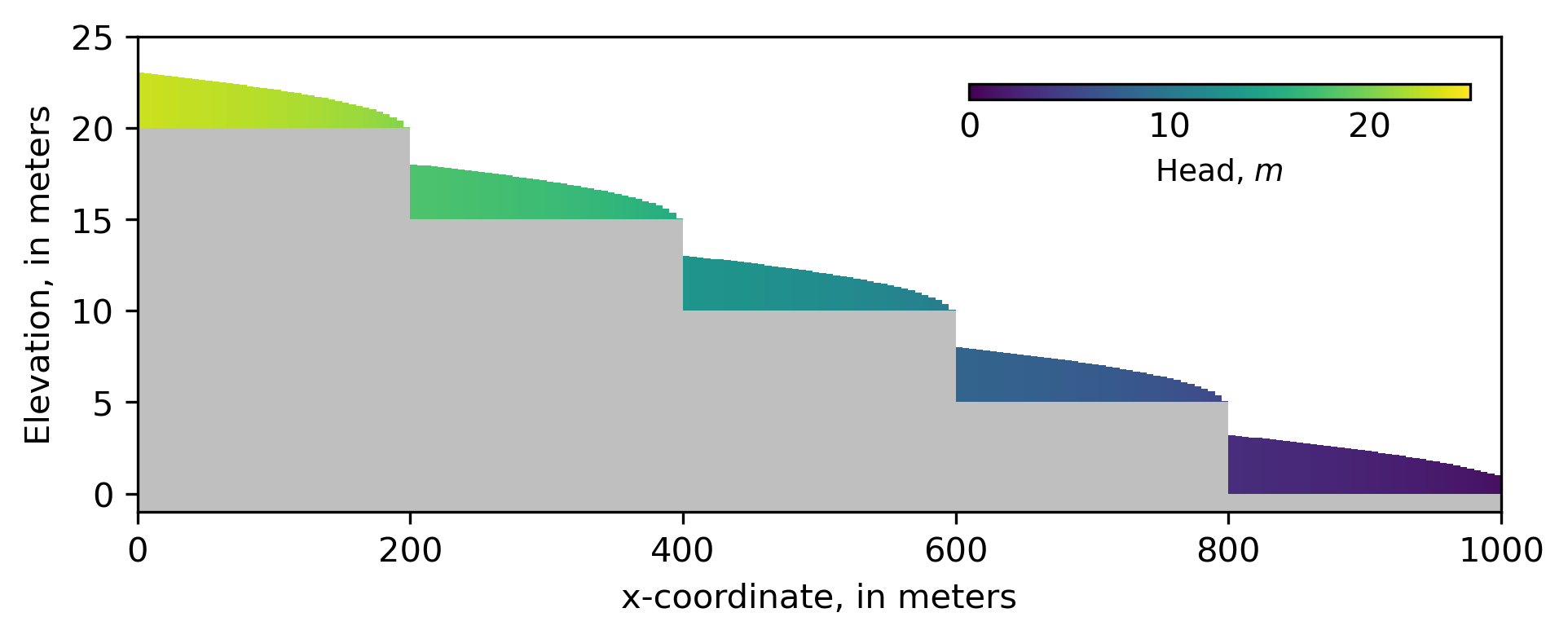
Let’s run the model and plot the heads. We should (hopefully) see a converged solution and a fun stair-stepping pattern in heads.

run_model()
plot_results(plot_head=True)

<flopy.mf6.data.mfstructure.MFDataItemStructure object at 0x7f8ae09bea10>
writing simulation...
  writing simulation name file...
  writing simulation tdis package...
  writing solution package ims_-1...
  writing model ex-gwf-zaidel...
    writing model name file...
    writing package dis...
    writing package npf...
    writing package ic...
    writing package ghb_0...
INFORMATION: maxbound in ('', 'ghb', 'dimensions') changed to 2 based on size of stress_period_data
    writing package oc...
mf6
                                   MODFLOW 6
                U.S. GEOLOGICAL SURVEY MODULAR HYDROLOGIC MODEL
                        VERSION 6.8.0.dev0+a6a4984.dirty
                               ***DEVELOP MODE***

   MODFLOW 6 compiled Jun 01 2026 18:46:14 with Intel(R) Fortran Intel(R) 64
   Compiler Classic for applications running on Intel(R) 64, Version 2021.6.0
                             Build 20220226_000000

This software is preliminary or provisional and is subject to
revision. It is being provided to meet the need for timely best
science. The software has not received final approval by the U.S.
Geological Survey (USGS). No warranty, expressed or implied, is made
by the USGS or the U.S. Government as to the functionality of the
software and related material nor shall the fact of release
constitute any such warranty. The software is provided on the
condition that neither the USGS nor the U.S. Government shall be held
liable for any damages resulting from the authorized or unauthorized
use of the software.


 MODFLOW runs in SEQUENTIAL mode

 Run start date and time (yyyy/mm/dd hh:mm:ss): 2026/06/02 18:42:47

 Writing simulation list file: mfsim.lst
 Using Simulation name file: mfsim.nam

    Solving:  Stress period:     1    Time step:     1

 Run end date and time (yyyy/mm/dd hh:mm:ss): 2026/06/02 18:42:47
 Elapsed run time:  0.021 Seconds

 Normal termination of simulation.
loading simulation...
  loading simulation name file...
  loading tdis package...
  loading model gwf6...
    loading package dis...
    loading package npf...
    loading package ic...
    loading package ghb...
    loading package oc...
  loading solution package ex-gwf-zaidel...

Run mf6adj

Now let’s try a direct-head performance measure (PM) with the adjoint method. Because there is only one stress period, there is no need to add multiple PMs for the same location.

pm_fname = "zaidel_perfmeas.dat"
fpm = open(pl.Path(workspace) / pm_fname, "w")
pm_col = 190  # pm column
layer, row = 1, 1  # the layer row
sp, ts = 1, 1  # stress period and time step
pm_name = "pm_single"
fpm.write(f"begin performance_measure {pm_name}\n")
fpm.write(f"{sp} {ts} {layer} {row} {pm_col} head direct 1.0 -1e30\n")
fpm.write("end performance_measure\n\n")
fpm.close()

Now let’s run the adjoint solution. Recall this involves a single forward run of the model and then a solve of the adjoint state for each SP and TS, backwards in time.

forward_hdf5_name = "zaidel.hdf5"
start = datetime.now()
adj = mf6adj.Mf6Adj(
    pm_fname,
    lib_name,
    logging_level="INFO",
    working_directory=workspace,
)
adj.solve_forward_model(
    hdf5_name=forward_hdf5_name
)  # solve the standard forward solution
dfsum = adj.solve_adjoint()  # solve the adjoint state for each performance measure
adj.finalize()  # release components
duration = (datetime.now() - start).total_seconds()
print("took:", duration)

2026-06-02 18:42:47,443 - Logger instance 'Mf6Adj-zaidel_perfmeas-ebb7e314' created.
2026-06-02 18:42:47,443 - Running from /home/runner/work/mf6adj/mf6adj/examples/ex-gwf-zaidel
2026-06-02 18:42:47,444 - Structured grid found
2026-06-02 18:42:47,455 - MODFLOW 6 version: 6.8.0.dev0
2026-06-02 18:42:47,456 - Processing adjoint file: zaidel_perfmeas.dat
2026-06-02 18:42:47,458 - Starting flow solution
2026-06-02 18:42:47,467 - Flow (stress period,time step) (1,1) converged in 64 iters, took 0.00011905 mins
2026-06-02 18:42:47,472 - Flow solution finished and took 0.00022308 minutes
2026-06-02 18:42:47,478 - Starting solve_adjoint at 2026-06-02 18:42:47.478139
2026-06-02 18:42:47,481 - Structured grid found, shape: (1, 1, 200)
2026-06-02 18:42:47,483 - Starting adjoint solve for PerfMeas: pm_single (kper, kstp) (1, 1)
2026-06-02 18:42:47,484 - Solving for lambda
2026-06-02 18:42:47,485 - Solving with direct with solver options: {'use_umfpack': True}
2026-06-02 18:42:47,486 - Solving for lambda took: 0.001645 seconds
2026-06-02 18:42:47,489 - Adjoint solve took: 0.00652 seconds to solve adjoint solution for PerfMeas: pm_single (kper, kstp) (1, 1)
2026-06-02 18:42:47,490 - Write group to hdf file
2026-06-02 18:42:47,492 - Formulate composite sensitivities
2026-06-02 18:42:47,493 - Writing composite sensitivities
2026-06-02 18:42:47,496 - Adjoint solve took:   0.018577 seconds for pm 'pm_single' at (kper,kstp) (1, 1)
2026-06-02 18:42:47,497 - Finalizing Mf6Adj

took: 0.068925

Plot the Results

Looks like it ran, yay! Now let’s check out what output files are in the working directory. Recall, Mf6Adj stores outputs in a hierarchical data (HDF5) format. This is necessary because the adjoint solution would otherwise have to store quite a lot of information from the forward run (conductance, RHS, etc.) in memory. Plus, it avoids saving out the adjoint results to tons of ascii files that can clutter up the working directory fast.

[f for f in os.listdir(workspace) if f.endswith("hdf5")]

['adjoint_solution_pm_single.hdf5', 'zaidel.hdf5']

The Zaidel HDF5 file contains the forward-run components, whereas the adjoint-solution HDF5 file contains the outputs we want. Let’s look at what is in the results file. It should include all timesteps and stress periods for all performance measures, which in this case is just one.

result_hdf = "adjoint_solution_pm_single.hdf5"
hdf = h5py.File(pl.Path(workspace) / result_hdf, "r")
keys = list(hdf.keys())
keys.sort()
keys

['composite', 'solution_kper:00000_kstp:00000']

Now let’s investigate the components for which we have sensitivity results for that direct head PM. There should be one for every BC parameter in the model, as well as K components.

grp = hdf["composite"]
plot_keys = [i for i in grp.keys() if len(grp[i].shape) == 3]
plot_keys

['ghb_0_bhead', 'ghb_0_cond', 'k11', 'k33', 'rch6_recharge', 'wel6_q']

But wait! There are results for two extra BCs that were not part of the Zaidel model: the recharge and well package. Why is that?

This is because the adjoint state is equivalent to the sensitivity of the PM to a unit injection of water in every cell. A unit injection of water is equivalent to a specified-flux BC, such as recharge or a well (assuming Q is positive for injection in the well package).

So for any Mf6Adj solution, you automatically get the sensitivity of the PM to recharge and well Q regardless of them being in the model.

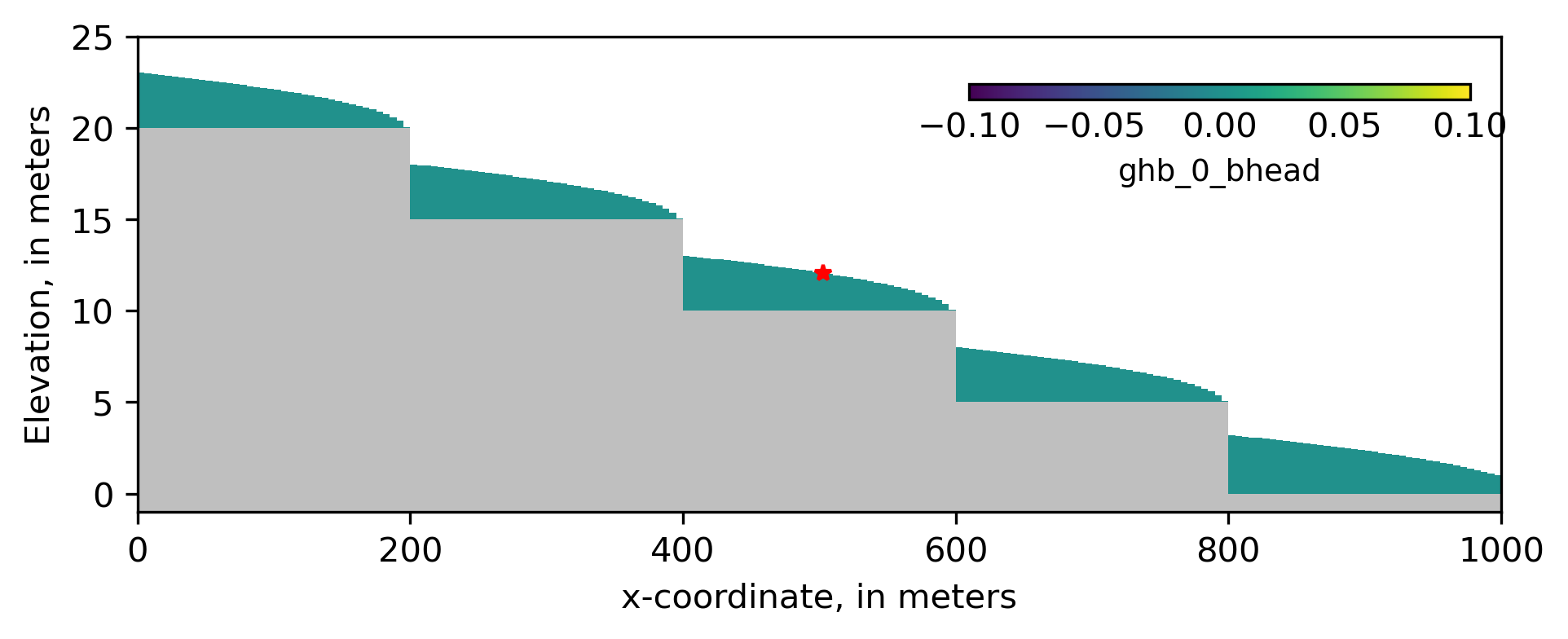
All right, now let’s plot up the results and see if they make sense. Let’s start with the GHB parameters: GHB head and conductance.

keys = [pkey for pkey in plot_keys if "ghb" in pkey]
for pkey in keys:
    arr = grp[pkey][:]
    for k, karr in enumerate(arr):
        plot_results(
            arr=karr, plot_head=False, arr_label=pkey, plot_pm=True, pm_col=pm_col
        )

loading simulation...
  loading simulation name file...
  loading tdis package...
  loading model gwf6...
    loading package dis...
    loading package npf...
    loading package ic...
    loading package ghb...
    loading package oc...
  loading solution package ex-gwf-zaidel...
loading simulation...
  loading simulation name file...
  loading tdis package...
  loading model gwf6...
    loading package dis...
    loading package npf...
    loading package ic...
    loading package ghb...
    loading package oc...
  loading solution package ex-gwf-zaidel...

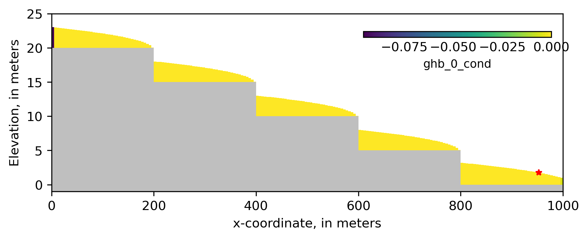
Cool! The adjoint results show that the head PM is more sensitive to GHB head than conductance. That makes intuitive sense, since conductance is much larger than head in this example and typically varies over a larger scale, so heads would be less responsive to a unit change in conductance.

Another interesting result is in the relative sensitivities of the upgradient and downgradient GHBs. For GHB head, it makes sense that head in column 190 would be more sensitive to the downgradient GHB.

But why does the downgradient GHB show a negative sensitivity value and the upgradient GHB a positive sensitivity value?

The adjoint method solves for the response of the PM to a positive increment in the parameter. For the upgradient GHB, a higher conductance means slightly more flux into the domain and a higher downgradient head. For the downgradient GHB, a higher conductance tends to flatten the water table at the lowest step, leading to a slightly lower head at the PM. Conductance up, head up is a positive sensitivity; conductance up, head down is a negative sensitivity.

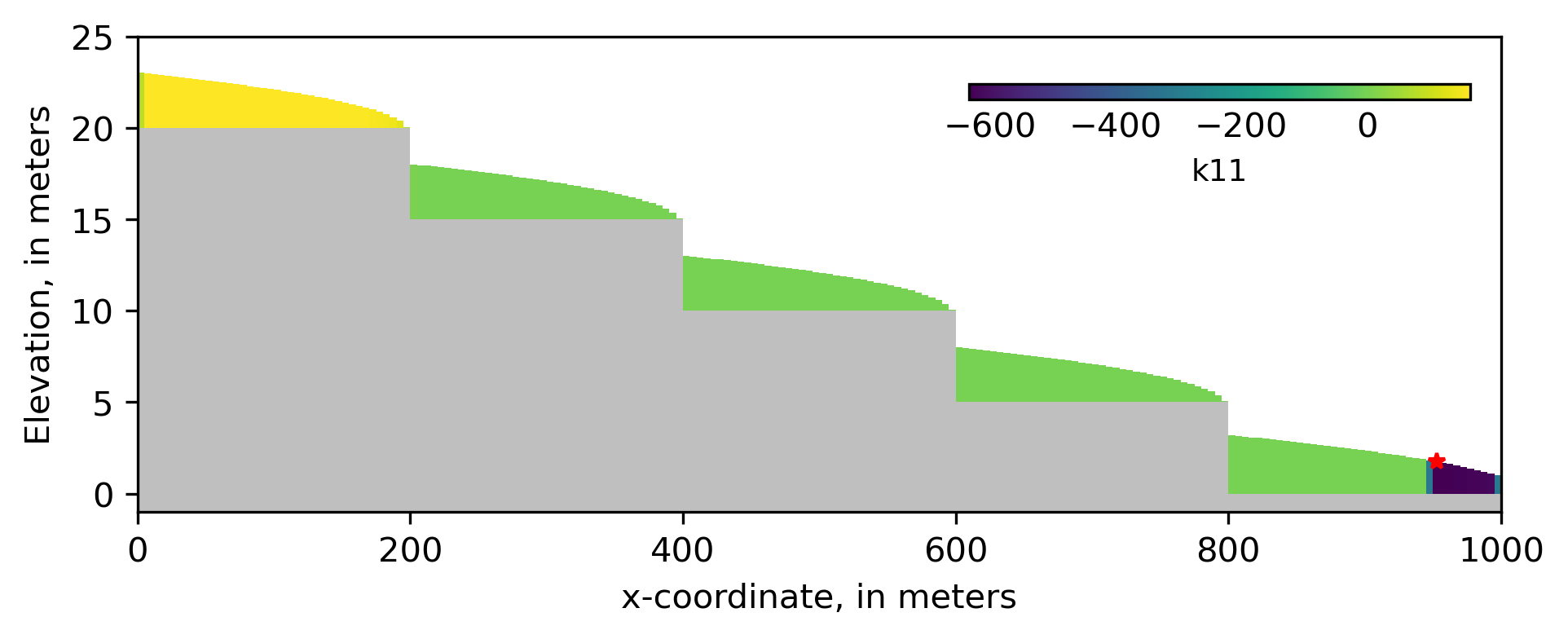
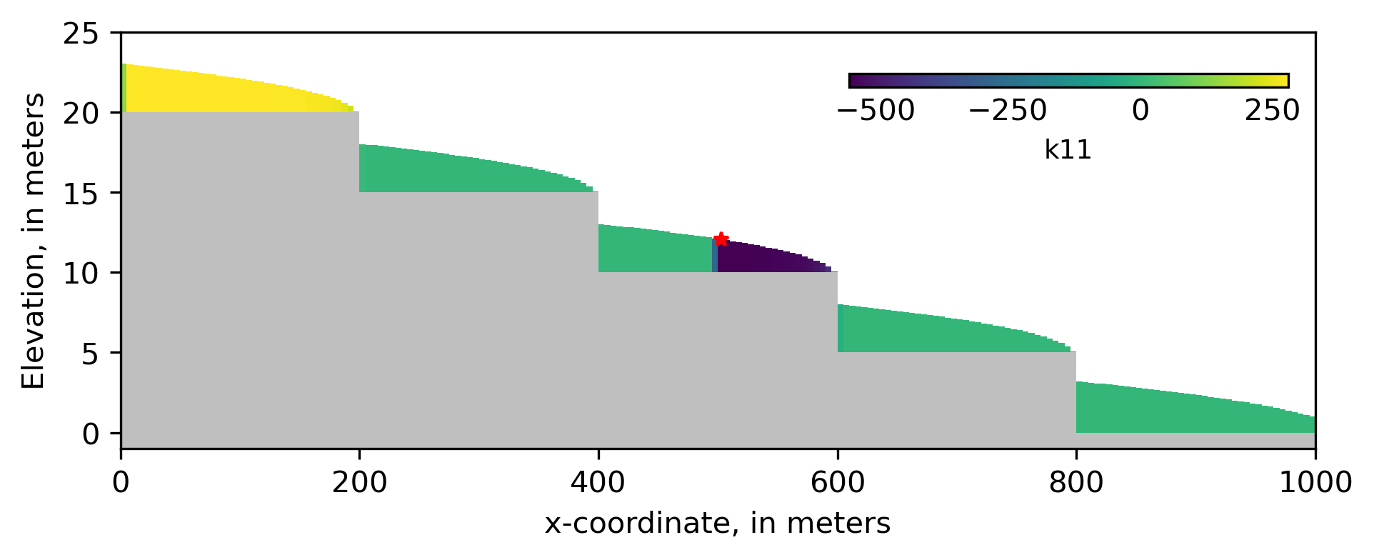
Now let’s take a look at the components of K: K11 and K33 (horizontal and vertical K)

keys = [pkey for pkey in plot_keys if "k" in pkey]
for pkey in keys:
    arr = grp[pkey][:]
    for k, karr in enumerate(arr):
        plot_results(
            arr=karr, plot_head=False, arr_label=pkey, plot_pm=True, pm_col=pm_col
        )

loading simulation...
  loading simulation name file...
  loading tdis package...
  loading model gwf6...
    loading package dis...
    loading package npf...
    loading package ic...
    loading package ghb...
    loading package oc...
  loading solution package ex-gwf-zaidel...
loading simulation...
  loading simulation name file...
  loading tdis package...
  loading model gwf6...
    loading package dis...
    loading package npf...
    loading package ic...
    loading package ghb...
    loading package oc...
  loading solution package ex-gwf-zaidel...

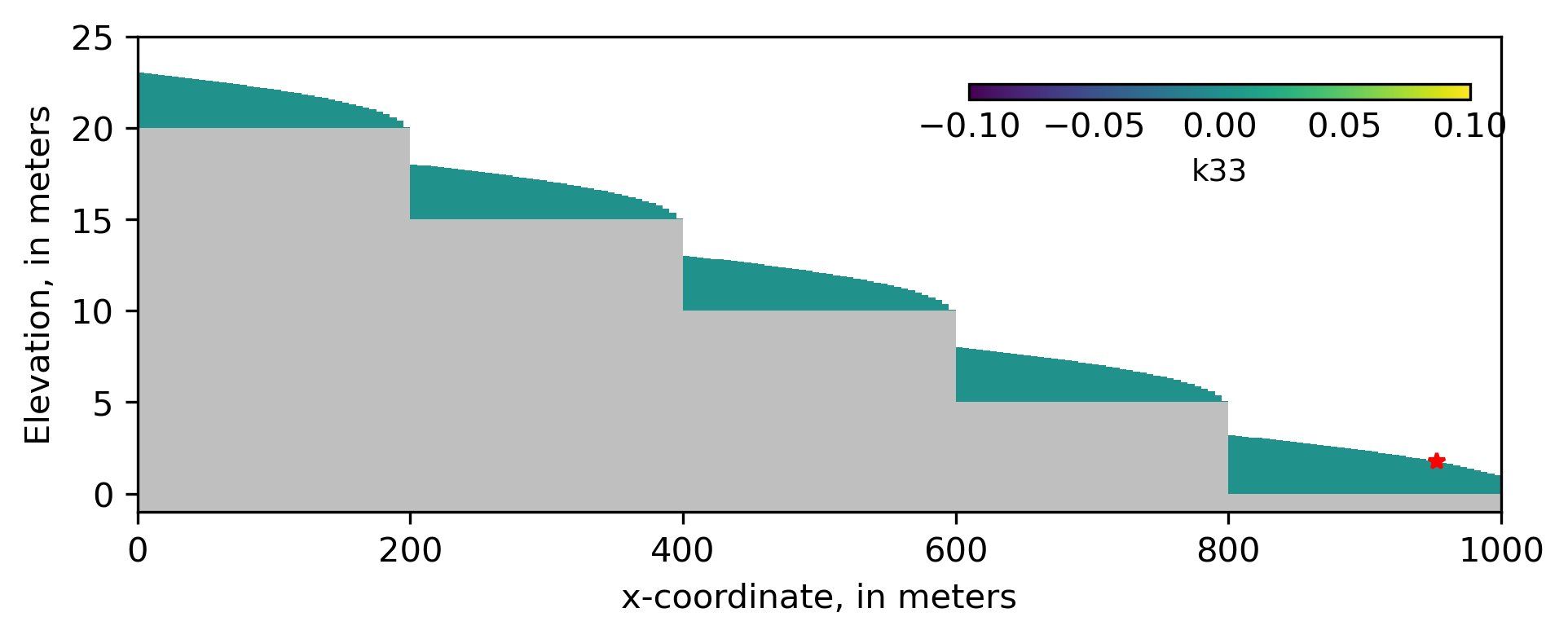
Wait, why is K33 zero sensitivity everywhere?

Because it is a one-layer model.

So what’s up with the zonal behavior with K11?

Just like with the GHB conductance, a higher K at the upgradient step containing the GHB leads to more flow into the domain and a higher head PM. A higher K downgradient of the PM (but on the same step) would act to flatten the water table and lead to a lower head PM. K values at the GHB locations have lower absolute sensitivities, reflecting the dominance of the BC conductance in those cells. Interestingly, horizontal K at all of the intervening upgradient steps has very small (but not zero) positive sensitivity. This reflects the fact that the heads in the Zaidel problem are largely governed by the GHBs.

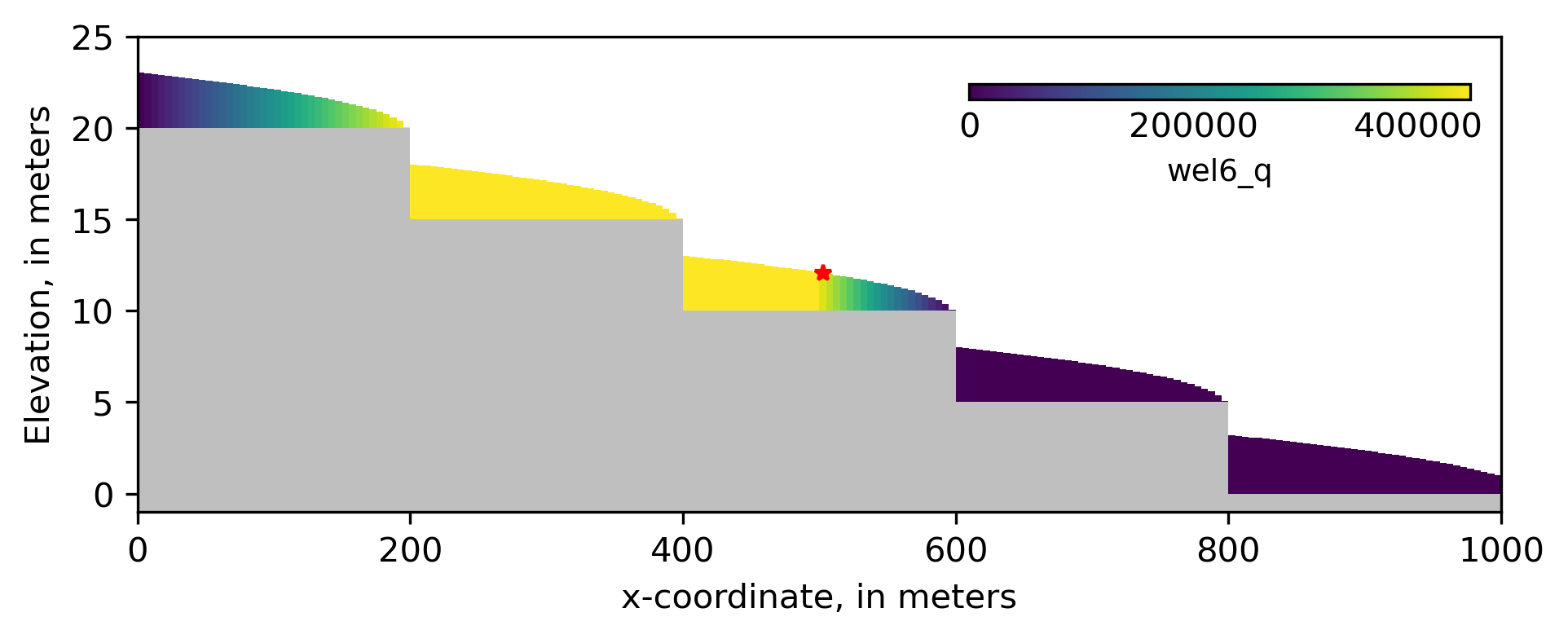
Last but not least, let’s take a look at the recharge and well results.

keys = [pkey for pkey in plot_keys if "rch" in pkey or "wel" in pkey]
for pkey in keys:
    arr = grp[pkey][:]
    for k, karr in enumerate(arr):
        plot_results(
            arr=karr, plot_head=False, arr_label=pkey, plot_pm=True, pm_col=pm_col
        )

loading simulation...
  loading simulation name file...
  loading tdis package...
  loading model gwf6...
    loading package dis...
    loading package npf...
    loading package ic...
    loading package ghb...
    loading package oc...
  loading solution package ex-gwf-zaidel...
loading simulation...
  loading simulation name file...
  loading tdis package...
  loading model gwf6...
    loading package dis...
    loading package npf...
    loading package ic...
    loading package ghb...
    loading package oc...
  loading solution package ex-gwf-zaidel...

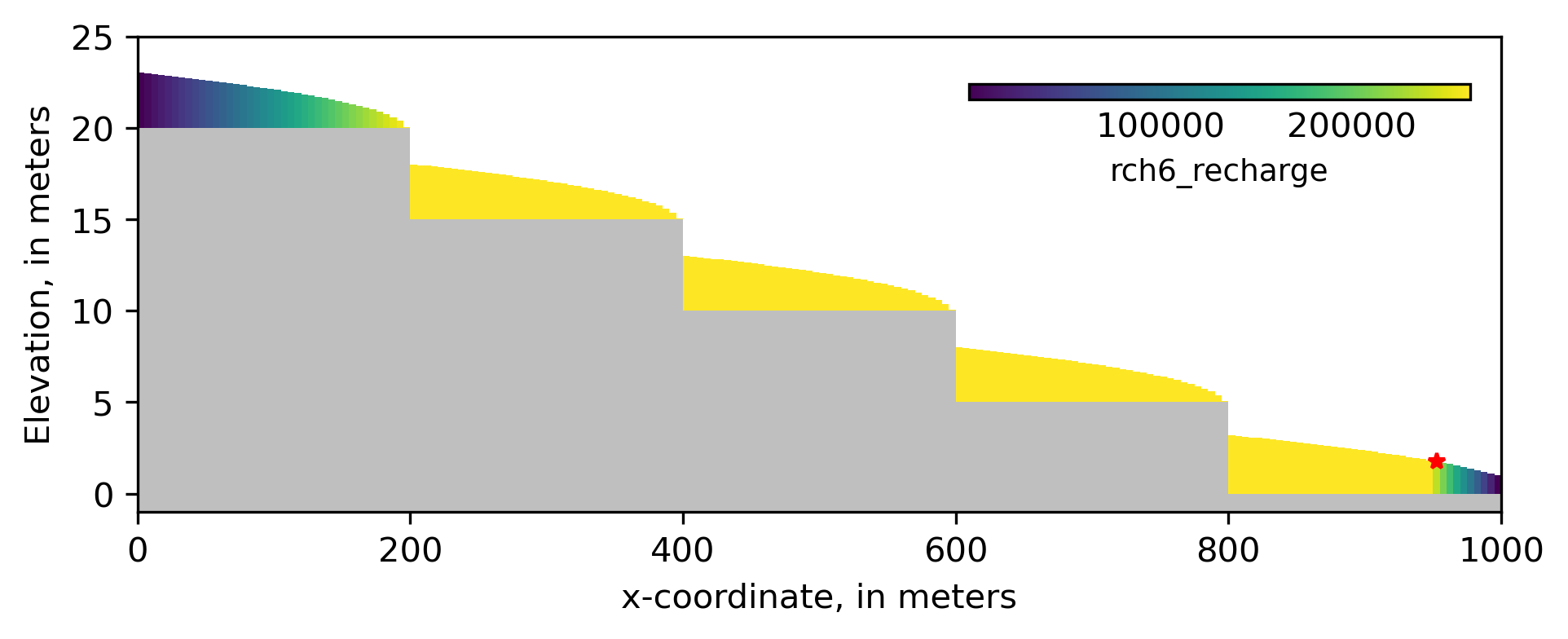
As expected, they are identical. This is because neither package exists in the model, and so they reflect the sensitivity of the direct head PM to a unit injection of water. But let’s unpack these results a bit further…

Recharge/well Q downgradient of the PM shows decreasing sensitivity the further you move away from the PM. Because the problem is discontinuous, we would expect that sensitivity to drop to zero at the next lower stair step to the head PM. Conversely, upgradient sensitivity is uniformly high until the furthest upgradient step is reached, where the sensitivity drops lower as it approaches the upgradient GHB. This reflects the interplay between unit injection of water and the fixed GHB head.

Let’s test our adjoint intuition a bit. What happens if we put the direct-head PM in the middle of the domain?

Self-study: Walk through the results and try to explain the differences you see relative to the previous case.

# close previous hdf5 connection
hdf.close()

# build and run model
run_model()

# build PM input
pm_col = 100  # pm column
pm_fname = "zaidel_perfmeas.dat"
fpm = open(pl.Path(workspace) / pm_fname, "w")

layer, row = 1, 1  # the layer row and column
sp, ts = 1, 1  # stress period and time step
pm_name = "pm_single"
fpm.write(f"begin performance_measure {pm_name}\n")
fpm.write(f"{sp} {ts} {layer} {row} {pm_col} head direct 1.0 -1e30\n")
fpm.write("end performance_measure\n\n")
fpm.close()

# run adjoint
forward_hdf5_name = "zaidel.hdf5"
start = datetime.now()

adj = mf6adj.Mf6Adj(
    pm_fname,
    lib_name,
    logging_level="INFO",
    working_directory=workspace,
)
adj.solve_forward_model(
    hdf5_name=forward_hdf5_name
)  # solve the standard forward solution
dfsum = adj.solve_adjoint()  # solve the adjoint state for each performance measure
adj.finalize()  # release components
duration = (datetime.now() - start).total_seconds()
print("took:", duration)

2026-06-02 18:42:49,178 - Logger instance 'Mf6Adj-zaidel_perfmeas-3c97855f' created.
2026-06-02 18:42:49,179 - Running from /home/runner/work/mf6adj/mf6adj/examples/ex-gwf-zaidel
2026-06-02 18:42:49,180 - Structured grid found
2026-06-02 18:42:49,186 - MODFLOW 6 version: 6.8.0.dev0
2026-06-02 18:42:49,187 - Processing adjoint file: zaidel_perfmeas.dat
2026-06-02 18:42:49,188 - Starting flow solution
2026-06-02 18:42:49,197 - Flow (stress period,time step) (1,1) converged in 64 iters, took 0.00011727 mins
2026-06-02 18:42:49,201 - Flow solution finished and took 0.00021088 minutes
2026-06-02 18:42:49,206 - Starting solve_adjoint at 2026-06-02 18:42:49.206897
2026-06-02 18:42:49,207 - Removing existing adjoint solution file 'adjoint_solution_pm_single.hdf5'
2026-06-02 18:42:49,210 - Structured grid found, shape: (1, 1, 200)
2026-06-02 18:42:49,212 - Starting adjoint solve for PerfMeas: pm_single (kper, kstp) (1, 1)
2026-06-02 18:42:49,214 - Solving for lambda
2026-06-02 18:42:49,216 - Solving with direct with solver options: {'use_umfpack': True}
2026-06-02 18:42:49,217 - Solving for lambda took: 0.002757 seconds
2026-06-02 18:42:49,220 - Adjoint solve took: 0.007918 seconds to solve adjoint solution for PerfMeas: pm_single (kper, kstp) (1, 1)
2026-06-02 18:42:49,221 - Write group to hdf file
2026-06-02 18:42:49,224 - Formulate composite sensitivities
2026-06-02 18:42:49,224 - Writing composite sensitivities
2026-06-02 18:42:49,227 - Adjoint solve took:   0.020932 seconds for pm 'pm_single' at (kper,kstp) (1, 1)
2026-06-02 18:42:49,228 - Finalizing Mf6Adj

<flopy.mf6.data.mfstructure.MFDataItemStructure object at 0x7f8ae09bea10>
writing simulation...
  writing simulation name file...
  writing simulation tdis package...
  writing solution package ims_-1...
  writing model ex-gwf-zaidel...
    writing model name file...
    writing package dis...
    writing package npf...
    writing package ic...
    writing package ghb_0...
INFORMATION: maxbound in ('', 'ghb', 'dimensions') changed to 2 based on size of stress_period_data
    writing package oc...
mf6
                                   MODFLOW 6
                U.S. GEOLOGICAL SURVEY MODULAR HYDROLOGIC MODEL
                        VERSION 6.8.0.dev0+a6a4984.dirty
                               ***DEVELOP MODE***

   MODFLOW 6 compiled Jun 01 2026 18:46:14 with Intel(R) Fortran Intel(R) 64
   Compiler Classic for applications running on Intel(R) 64, Version 2021.6.0
                             Build 20220226_000000

This software is preliminary or provisional and is subject to
revision. It is being provided to meet the need for timely best
science. The software has not received final approval by the U.S.
Geological Survey (USGS). No warranty, expressed or implied, is made
by the USGS or the U.S. Government as to the functionality of the
software and related material nor shall the fact of release
constitute any such warranty. The software is provided on the
condition that neither the USGS nor the U.S. Government shall be held
liable for any damages resulting from the authorized or unauthorized
use of the software.


 MODFLOW runs in SEQUENTIAL mode

 Run start date and time (yyyy/mm/dd hh:mm:ss): 2026/06/02 18:42:49

 Writing simulation list file: mfsim.lst
 Using Simulation name file: mfsim.nam

    Solving:  Stress period:     1    Time step:     1

 Run end date and time (yyyy/mm/dd hh:mm:ss): 2026/06/02 18:42:49
 Elapsed run time:  0.022 Seconds

 Normal termination of simulation.
took: 0.064472

# get results and plot
result_hdf = "adjoint_solution_pm_single.hdf5"
hdf = h5py.File(pl.Path(workspace) / result_hdf, "r")
keys = list(hdf.keys())
keys.sort()
keys

['composite', 'solution_kper:00000_kstp:00000']

grp = hdf["composite"]
plot_keys = [i for i in grp.keys() if len(grp[i].shape) == 3]
for pkey in plot_keys:
    arr = grp[pkey][:]
    for k, karr in enumerate(arr):
        plot_results(
            arr=karr, plot_head=False, arr_label=pkey, plot_pm=True, pm_col=pm_col
        )

loading simulation...
  loading simulation name file...
  loading tdis package...
  loading model gwf6...
    loading package dis...
    loading package npf...
    loading package ic...
    loading package ghb...
    loading package oc...
  loading solution package ex-gwf-zaidel...
loading simulation...
  loading simulation name file...
  loading tdis package...
  loading model gwf6...
    loading package dis...
    loading package npf...
    loading package ic...
    loading package ghb...
    loading package oc...
  loading solution package ex-gwf-zaidel...
loading simulation...
  loading simulation name file...
  loading tdis package...
  loading model gwf6...
    loading package dis...
    loading package npf...
    loading package ic...
    loading package ghb...
    loading package oc...
  loading solution package ex-gwf-zaidel...
loading simulation...
  loading simulation name file...
  loading tdis package...
  loading model gwf6...
    loading package dis...
    loading package npf...
    loading package ic...
    loading package ghb...
    loading package oc...
  loading solution package ex-gwf-zaidel...
loading simulation...
  loading simulation name file...
  loading tdis package...
  loading model gwf6...
    loading package dis...
    loading package npf...
    loading package ic...
    loading package ghb...
    loading package oc...
  loading solution package ex-gwf-zaidel...
loading simulation...
  loading simulation name file...
  loading tdis package...
  loading model gwf6...
    loading package dis...
    loading package npf...
    loading package ic...
    loading package ghb...
    loading package oc...
  loading solution package ex-gwf-zaidel...

This example demonstrates how much information can be obtained by running Mf6Adj for a single direct-head performance measure on a simple 2-D steady-state model.

The same approach can be even more valuable for larger, more complex modeling applications, all for the computational cost of a single forward run and a single adjoint solution.