mf6adj demonstration using a simple box model
In this notebook, we test mf6adj on a simple box problem and compare the results with an analytical solution.
Import Packages
[1]:
import os
import pathlib as pl
import platform
import shutil
import sys
from datetime import datetime

import flopy
import h5py
import matplotlib.pyplot as plt
import numpy as np
import pandas as pd
import pyemu

try:
    import mf6adj
except ImportError:
    sys.path.insert(0, str(pl.Path("../").resolve()))
    import mf6adj
[2]:
mf6_bin, lib_name = mf6adj.get_conda_mf6_paths()
print(f"Using MF6 binary: {mf6_bin}")
print(f"Using MF6 library: {lib_name}")
Using MF6 binary: /home/runner/work/mf6adj/mf6adj/.pixi/envs/default/bin/mf6
Using MF6 library: /home/runner/work/mf6adj/mf6adj/.pixi/envs/default/bin/libmf6.so
Copy the MODFLOW Model
[3]:
org_ws = pl.Path("xd_box_chd_ana")
assert pl.Path(org_ws).exists()
Set up a local copy of the model files.
[4]:
ws = pl.Path("xd_box_chd_ana_working")
if pl.Path(ws).exists():
    shutil.rmtree(ws)
shutil.copytree(org_ws, ws)
[4]:
PosixPath('xd_box_chd_ana_working')
[5]:
sim = flopy.mf6.MFSimulation.load(sim_ws=ws)
m = sim.get_model()
loading simulation...
  loading simulation name file...
  loading tdis package...
  loading model gwf6...
    loading package dis...
    loading package ic...
    loading package sto...
    loading package chd...
    loading package wel...
    loading package oc...
    loading package npf...
  loading solution package xdbox...
[6]:
ib = m.dis.idomain.array[0, :, :].astype(float)
ib[ib > 0] = np.nan
ib_cmap = plt.get_cmap("Greys_r")
ib_cmap.set_bad(alpha=0.0)


def plot_model(arr, units=None):
    arr[~np.isnan(ib)] = np.nan
    fig, ax = plt.subplots(1, 1, figsize=(6, 6))
    cb = ax.imshow(arr, cmap="plasma")
    plt.colorbar(cb, ax=ax, label=units)
    plt.imshow(ib, cmap=ib_cmap)
    return fig, ax
Run the existing model in our local workspace.
[7]:
print(mf6_bin)
print(ws)
print(os.listdir(ws))
pyemu.os_utils.run(mf6_bin.name, cwd=ws)
/home/runner/work/mf6adj/mf6adj/.pixi/envs/default/bin/mf6
xd_box_chd_ana_working
['xdbox.tdis', 'xdbox.dis', 'xdbox.chd', 'xdbox.sto', 'xdbox.cbb', 'xdbox.oc', 'mfsim.nam', 'xdbox.nam', 'test.adj', 'xdbox.ims', 'xdbox.npf', 'xdbox.ic', 'xdbox.wel']
mf6
                                   MODFLOW 6
                U.S. GEOLOGICAL SURVEY MODULAR HYDROLOGIC MODEL
                        VERSION 6.8.0.dev0+a6a4984.dirty
                               ***DEVELOP MODE***

   MODFLOW 6 compiled Jun 01 2026 18:46:14 with Intel(R) Fortran Intel(R) 64
   Compiler Classic for applications running on Intel(R) 64, Version 2021.6.0
                             Build 20220226_000000

This software is preliminary or provisional and is subject to
revision. It is being provided to meet the need for timely best
science. The software has not received final approval by the U.S.
Geological Survey (USGS). No warranty, expressed or implied, is made
by the USGS or the U.S. Government as to the functionality of the
software and related material nor shall the fact of release
constitute any such warranty. The software is provided on the
condition that neither the USGS nor the U.S. Government shall be held
liable for any damages resulting from the authorized or unauthorized
use of the software.


 MODFLOW runs in SEQUENTIAL mode

 Run start date and time (yyyy/mm/dd hh:mm:ss): 2026/06/02 18:36:46

 Writing simulation list file: mfsim.lst
 Using Simulation name file: mfsim.nam

    Solving:  Stress period:     1    Time step:     1

 Run end date and time (yyyy/mm/dd hh:mm:ss): 2026/06/02 18:36:46
 Elapsed run time:  0.143 Seconds

 Normal termination of simulation.
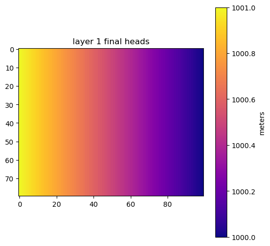
Now plot some heads.
[8]:
hds = flopy.utils.HeadFile(pl.Path(ws) / "xdbox.hds")
final_arr = hds.get_data()
fig, ax = plot_model(final_arr[0, :, :], units="meters")
ax.set_title("layer 1 final heads")
[8]:
Text(0.5, 1.0, 'layer 1 final heads')
The main requirement for using mf6adj is an input file that describes the performance measures. Fortunately, this file follows a modern format similar to other MF6 input files.
[9]:
pm_fname = "xdbox.dat"
fpm = open(pl.Path(ws) / pm_fname, "w")
Run mf6adj
[10]:
l, r, c = 1, 41, 21  # the layer row and column
sp, ts = 1, 1  # stress period and time step
pm_name = "pm_single"
fpm.write(f"begin performance_measure {pm_name}\n")
fpm.write(f"{sp} {ts} {l} {r} {c} head direct 1.0 -1e30\n")
fpm.write("end performance_measure\n\n")
fpm.close()
Now we should be ready to go. The adjoint solution process requires one forward model run and then a solve for the adjoint state, which uses the forward solution components (for example, the conductance matrix, RHS, heads, and saturation). The adjoint solve has two important characteristics: it is linear, regardless of the forward model’s linearity, and it proceeds backward in time, starting with the last stress period.
[11]:
forward_hdf5_name = "forward.hdf5"
start = datetime.now()
import mf6adj

adj = mf6adj.Mf6Adj(pm_fname, lib_name, logging_level="INFO", working_directory=ws)
adj.solve_forward_model(
    hdf5_name=forward_hdf5_name
)  # solve the standard forward solution
dfsum = adj.solve_adjoint()  # solve the adjoint state for each performance measure
adj.finalize()  # release components
duration = (datetime.now() - start).total_seconds()
print("took:", duration)
2026-06-02 18:36:46,673 - Logger instance 'Mf6Adj-xdbox-71a8a691' created.
2026-06-02 18:36:46,674 - Running from /home/runner/work/mf6adj/mf6adj/examples/xd_box_chd_ana_working
2026-06-02 18:36:46,675 - Structured grid found
2026-06-02 18:36:46,696 - MODFLOW 6 version: 6.8.0.dev0
2026-06-02 18:36:46,697 - Processing adjoint file: xdbox.dat
2026-06-02 18:36:46,698 - Starting flow solution
2026-06-02 18:36:46,791 - Flow (stress period,time step) (1,1) converged in 2 iters, took   0.001519 mins
2026-06-02 18:36:46,819 - Flow solution finished and took  0.0020078 minutes
2026-06-02 18:36:46,828 - Starting solve_adjoint at 2026-06-02 18:36:46.828952
2026-06-02 18:36:46,831 - Structured grid found, shape: (1, 80, 100)
2026-06-02 18:36:46,834 - Starting adjoint solve for PerfMeas: pm_single (kper, kstp) (1, 1)
2026-06-02 18:36:46,836 - Solving for lambda
2026-06-02 18:36:46,837 - Solving with direct with solver options: {'use_umfpack': True}
2026-06-02 18:36:46,858 - Solving for lambda took: 0.021637 seconds
2026-06-02 18:36:46,963 - Adjoint solve took: 0.128761 seconds to solve adjoint solution for PerfMeas: pm_single (kper, kstp) (1, 1)
2026-06-02 18:36:46,963 - Write group to hdf file
2026-06-02 18:36:46,983 - Formulate composite sensitivities
2026-06-02 18:36:46,983 - Writing composite sensitivities
2026-06-02 18:36:46,996 - Adjoint solve took:    0.16794 seconds for pm 'pm_single' at (kper,kstp) (1, 1)
2026-06-02 18:36:46,997 - Finalizing Mf6Adj
took: 0.351643
Let’s see what happened.
Plot the Results
[12]:
[f for f in os.listdir(ws) if f.endswith("hdf5")]
[12]:
['forward.hdf5', 'adjoint_solution_pm_single.hdf5']
mf6adj uses the widely available HDF5 format to store information. These files hold low-level details about the adjoint solution. However, mf6adj.solve_adjoint() also returns a higher-level summary of the results. Let’s look at that first.
[13]:
type(dfsum)
[13]:
dict
[14]:
list(dfsum.keys())
[14]:
['pm_single']
[15]:
dfhw = dfsum["pm_single"]
dfhw
[15]:
| k11 | k33 | wel6_q | rch6_recharge | ss | |
|---|---|---|---|---|---|
| node | |||||
| 1 | 0.000003 | 0.0 | 0.000000 | 0.000000 | 0.000000 |
| 2 | 0.000005 | 0.0 | 0.000543 | 0.000543 | -0.000066 |
| 3 | 0.000005 | 0.0 | 0.001084 | 0.001084 | -0.000130 |
| 4 | 0.000005 | 0.0 | 0.001622 | 0.001622 | -0.000190 |
| 5 | 0.000005 | 0.0 | 0.002156 | 0.002156 | -0.000247 |
| ... | ... | ... | ... | ... | ... |
| 7996 | -0.000002 | 0.0 | 0.000959 | 0.000959 | 0.000110 |
| 7997 | -0.000002 | 0.0 | 0.000719 | 0.000719 | 0.000084 |
| 7998 | -0.000002 | 0.0 | 0.000480 | 0.000480 | 0.000057 |
| 7999 | -0.000002 | 0.0 | 0.000240 | 0.000240 | 0.000029 |
| 8000 | -0.000001 | 0.0 | 0.000000 | 0.000000 | 0.000000 |
8000 rows × 5 columns
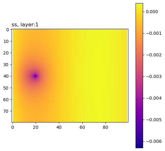
Those are the node-scale sensitivities for the selected performance measure. Plotting them is easiest using the HDF5 file itself.
[16]:
result_hdf = "adjoint_solution_pm_single.hdf5"
hdf = h5py.File(pl.Path(ws) / result_hdf, "r")
keys = list(hdf.keys())
keys.sort()
print(keys)
['composite', 'solution_kper:00000_kstp:00000']
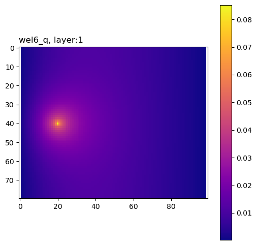
The composite group contains sensitivities of the performance measure to the model inputs, summed across all adjoint solutions.
[17]:
grp = hdf["composite"]
plot_keys = [i for i in grp.keys() if len(grp[i].shape) == 3]
plot_keys
grp["wel6_q"][:]
[17]:
array([[[0.        , 0.00054254, 0.0010837 , ..., 0.00047285,
         0.00023644, 0.        ],
        [0.        , 0.00054393, 0.00108647, ..., 0.00047291,
         0.00023647, 0.        ],
        [0.        , 0.00054671, 0.00109203, ..., 0.00047304,
         0.00023653, 0.        ],
        ...,
        [0.        , 0.00057099, 0.00114049, ..., 0.0004798 ,
         0.00023991, 0.        ],
        [0.        , 0.00056802, 0.00113457, ..., 0.0004797 ,
         0.00023986, 0.        ],
        [0.        , 0.00056654, 0.00113162, ..., 0.00047964,
         0.00023983, 0.        ]]], shape=(1, 80, 100))
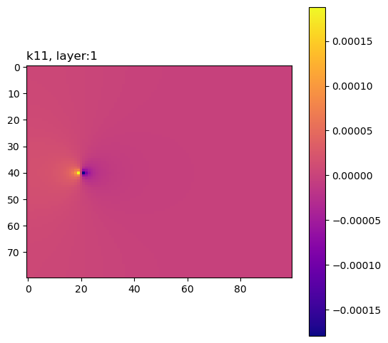
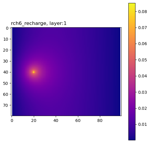
Here is a simple routine to plot these sensitivities.
[18]:
for pkey in plot_keys:
    arr = grp[pkey][:]
    for k, karr in enumerate(arr):
        karr[karr == 0.0] = np.nan
        fig, ax = plot_model(karr)
        ax.set_title(pkey + f", layer:{k + 1}", loc="left")
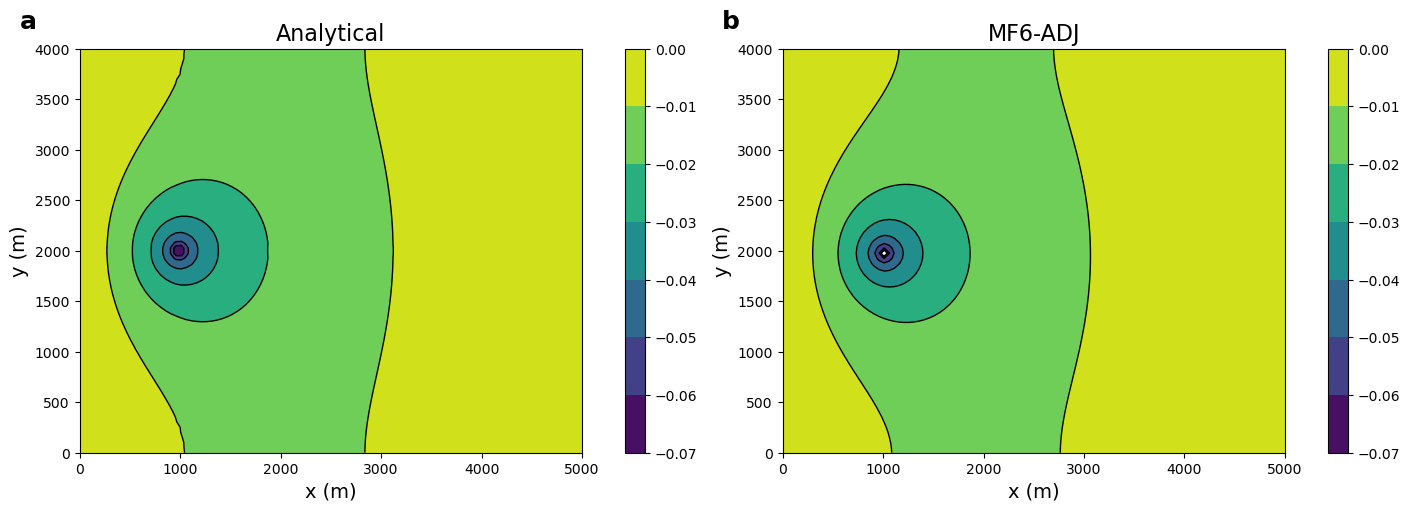
Define the analytical solution (Lu and Vesselinov, WRR, 2015; doi:10.1002/2014WR016819).
[19]:
H1, H2 = 1001.0, 1000.0  # Heads at both sides
L1, L2 = 500.0, 400.0  # Domain size
nlay, nrow, ncol = m.dis.nlay.data, m.dis.nrow.data, m.dis.ncol.data
delrow, delcol = m.dis.delr.data[0], m.dis.delc.data[0]
L1 = delrow * ncol
L2 = delcol * nrow
H = 1.0
k = 10.0  # Hydraulic conductivity
T = k * H  # Transmissivity
D = L1 * L2


def alpha(m):
    return m * np.pi / L1


def beta(n):
    return n * np.pi / L2


def omega_square(m, n):
    return (alpha(m)) ** 2 + (beta(n)) ** 2


def phi_s(x, y, xs, ys, M=5, N=5):
    listofmindices = [item + 1 for item in range(M)]
    Sum = 0.0
    a = [0.5]
    for i in [item + 1 for item in range(N)]:
        a.append(1.0)
    for n in range(N + 1):
        for m in listofmindices:
            Sum = Sum + a[n] * np.sin(alpha(m) * x) * np.cos(beta(n) * y) * np.sin(
                alpha(m) * xs
            ) * np.cos(beta(n) * ys) / omega_square(m, n)
    Sum = (4 / (T * D)) * Sum
    return Sum


def get_analytical_adj_state(xs, ys, M, N):
    list_adj_state = []
    for j in range(nrow):
        for i in range(ncol):
            x = m.modelgrid.xcellcenters[j][i]
            y = m.modelgrid.ycellcenters[j][i]
            list_adj_state.append(phi_s(x, y, xs, ys, M=M, N=N))
    array_adj_state = np.array(list_adj_state)
    print("array_adj_state = ", array_adj_state)
    filepath = pl.Path(ws) / "lamb_Analytical.txt"
    with open(filepath, "w") as file:
        # with open('lamb_Analytical.txt', 'w') as file:
        for value in array_adj_state:
            file.write(f"{value}\n")
    array_adj_state_2D = np.reshape(array_adj_state, (nrow, ncol))
    return array_adj_state_2D
[20]:
def plot_colorbar_contour(x, y, l_anal, l_num, vmin, vmax):
    _, axes = plt.subplots(1, 2, figsize=(14, 5), constrained_layout=True)
    ax = axes[0]
    ax.set_title("Analytical", fontsize=16)
    cs = ax.contourf(x, y, l_anal, zorder=1, vmin=vmin, vmax=vmax)
    ax.contour(cs, colors="k", linewidths=1.0, linestyles="-")
    plt.colorbar(cs)
    ax.set_xlabel("x (m)", fontsize=14)
    ax.set_ylabel("y (m)", fontsize=14)
    ax.text(-60.0, 420.0, "a", weight="bold", fontsize=18)
    plt.sca(ax)
    plt.xticks(
        [0, 100, 200, 300, 400, 500], ["0", "1000", "2000", "3000", "4000", "5000"]
    )
    plt.yticks(
        [0, 50, 100, 150, 200, 250, 300, 350, 400],
        ["0", "500", "1000", "1500", "2000", "2500", "3000", "3500", "4000"],
    )
    ax = axes[1]
    ax.set_title("MF6-ADJ", fontsize=16)
    cs = ax.contourf(x, y, l_num, zorder=1, vmin=vmin, vmax=vmax, levels=cs.levels)
    ax.contour(cs, colors="k", linewidths=1.0, linestyles="-")
    plt.colorbar(cs)
    ax.set_xlabel("x (m)", fontsize=14)
    ax.set_ylabel("y (m)", fontsize=14)
    ax.text(-60.0, 420.0, "b", weight="bold", fontsize=18)
    plt.sca(ax)
    plt.xticks(
        [0, 100, 200, 300, 400, 500], ["0", "1000", "2000", "3000", "4000", "5000"]
    )
    plt.yticks(
        [0, 50, 100, 150, 200, 250, 300, 350, 400],
        ["0", "500", "1000", "1500", "2000", "2500", "3000", "3500", "4000"],
    )
[21]:
# M & N should be large enough to get convergence
# of the analytical series solution (e.g., M=N=100)
lam_anal = get_analytical_adj_state(100.0, 200.0, M=100, N=100)
file_path = pl.Path(ws) / "lamb_Analytical.txt"
with open(file_path, "r") as file:
    lamb_ana = [float(line.strip()) for line in file]
    lamb_ana = np.array(lamb_ana)
    lamb_ana_arr = lamb_ana
    lamb_ana = np.reshape(lamb_ana, (nrow, ncol))
array_adj_state = [0.00028554 0.00085347 0.00142167 ... 0.00061386 0.00036824 0.00012284]
[22]:
lam_adj = grp["wel6_q"][:]
x = np.linspace(0, L1, ncol)
y = np.linspace(0, L2, nrow)
x_center = [x[i] + delcol / 2.0 for i in range(len(x))]
y_center = [y[i] + delrow / 2.0 for i in range(len(y))]
y = y[::-1]
y_center = y_center[::-1]
vmin, vmax = -lamb_ana.max(), -lamb_ana.min()
contour_intervals = np.arange(vmin, vmax, 0.003)
plot_colorbar_contour(x, y, -lamb_ana, -lam_adj[0], vmin, vmax)
[ ]: