mf6adj demonstration using the San Pedro model
In this notebook, we show how mf6adj can be used with a MODFLOW 6 version of the well-known San Pedro model of Leake et al. (2010).
Import Packages
[1]:
import os
import pathlib as pl
import platform
import shutil
import sys
from datetime import datetime

import flopy
import h5py
import matplotlib.pyplot as plt
import numpy as np
import pandas as pd
import pyemu
[2]:
try:
    import mf6adj
except ImportError:
    sys.path.insert(0, str(pl.Path("../").resolve()))
    import mf6adj
[3]:
mf6_bin, lib_name = mf6adj.get_conda_mf6_paths()
print(f"Using MF6 binary: {mf6_bin}")
print(f"Using MF6 library: {lib_name}")
Using MF6 binary: /home/runner/work/mf6adj/mf6adj/.pixi/envs/default/bin/mf6
Using MF6 library: /home/runner/work/mf6adj/mf6adj/.pixi/envs/default/bin/libmf6.so
Copy the MODFLOW Model
[4]:
org_ws = pl.Path("..") / "autotest" / "sanpedro" / "mf6_transient_ghb"
assert pl.Path(org_ws).exists()
Set up a local copy of the model files.
[5]:
ws = pl.Path("sanpedro")
if pl.Path(ws).exists():
    shutil.rmtree(ws)
shutil.copytree(org_ws, ws)
[5]:
PosixPath('sanpedro')
[6]:
sim = flopy.mf6.MFSimulation.load(sim_ws=ws)
m = sim.get_model()
loading simulation...
  loading simulation name file...
  loading tdis package...
  loading model gwf6...
    loading package dis...
    loading package rch...
    loading package ghb...
    loading package evt...
    loading package drn...
    loading package oc...
    loading package npf...
    loading package sto...
    loading package ic...
    loading package sfr...
  loading solution package sp_mf6...
[7]:
ib = m.dis.idomain.array.astype(float)
ib[ib > 0] = np.nan
ib[ib <= 0] = 0.5
ib_cmap = plt.get_cmap("Greys_r")
ib_cmap.set_bad(alpha=0.0)
X, Y = m.modelgrid.xcellcenters, m.modelgrid.ycellcenters
rdf = pd.DataFrame.from_records(m.sfr.packagedata.array)
rdf["i"] = rdf.cellid.apply(lambda x: int(x[1]))
rdf["j"] = rdf.cellid.apply(lambda x: int(x[2]))
sfr_arr = np.zeros((m.dis.nrow.data, m.dis.ncol.data))
sfr_arr[rdf.i, rdf.j] = 1
sfr_arr[sfr_arr == 0] = np.nan
sfr_cmap = plt.get_cmap("Blues")
sfr_cmap.set_bad(alpha=0.0)


def plot_model(k, arr, units=None, cmap="viridis"):
    arr[~np.isnan(ib[k, :, :])] = np.nan
    fig, ax = plt.subplots(1, 1, figsize=(6, 6))
    ax.set_aspect("equal")

    cb = ax.pcolormesh(X, Y, arr, cmap=cmap)
    plt.colorbar(cb, ax=ax, label=units)
    ax.pcolormesh(X, Y, ib[k, :, :], cmap=ib_cmap, alpha=0.5)
    ax.pcolormesh(X, Y, sfr_arr)
    ax.set_xticks([])
    ax.set_yticks([])
    return fig, ax
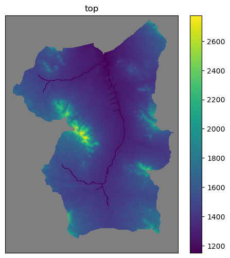
[8]:
# fig, ax = plot_model(4, m.dis.botm.array[4, :, :])
fig, ax = plot_model(4, m.dis.top.array)
_ = ax.set_title("top")
Run the existing model in our local workspace.
[9]:
pyemu.os_utils.run(mf6_bin.name, cwd=ws)
mf6
                                   MODFLOW 6
                U.S. GEOLOGICAL SURVEY MODULAR HYDROLOGIC MODEL
                        VERSION 6.8.0.dev0+a6a4984.dirty
                               ***DEVELOP MODE***

   MODFLOW 6 compiled Jun 01 2026 18:46:14 with Intel(R) Fortran Intel(R) 64
   Compiler Classic for applications running on Intel(R) 64, Version 2021.6.0
                             Build 20220226_000000

This software is preliminary or provisional and is subject to
revision. It is being provided to meet the need for timely best
science. The software has not received final approval by the U.S.
Geological Survey (USGS). No warranty, expressed or implied, is made
by the USGS or the U.S. Government as to the functionality of the
software and related material nor shall the fact of release
constitute any such warranty. The software is provided on the
condition that neither the USGS nor the U.S. Government shall be held
liable for any damages resulting from the authorized or unauthorized
use of the software.


 MODFLOW runs in SEQUENTIAL mode

 Run start date and time (yyyy/mm/dd hh:mm:ss): 2026/06/02 18:35:04

 Writing simulation list file: mfsim.lst
 Using Simulation name file: mfsim.nam

    Solving:  Stress period:     1    Time step:     1
    Solving:  Stress period:     1    Time step:     2
    Solving:  Stress period:     1    Time step:     3
    Solving:  Stress period:     1    Time step:     4
    Solving:  Stress period:     1    Time step:     5
    Solving:  Stress period:     1    Time step:     6
    Solving:  Stress period:     1    Time step:     7
    Solving:  Stress period:     1    Time step:     8
    Solving:  Stress period:     1    Time step:     9
    Solving:  Stress period:     1    Time step:    10

 Run end date and time (yyyy/mm/dd hh:mm:ss): 2026/06/02 18:35:15
 Elapsed run time: 11.032 Seconds

 Normal termination of simulation.
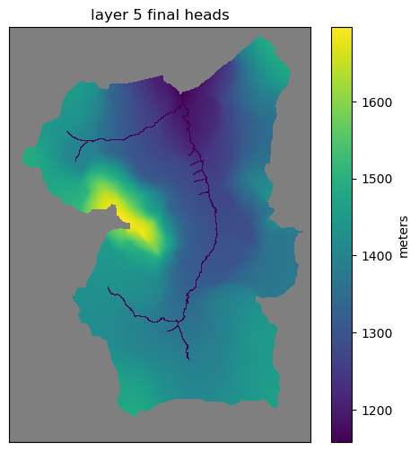
Now plot some heads.
[10]:
hds = flopy.utils.HeadFile(pl.Path(ws) / "sp_mf6.hds")
final_arr = hds.get_data()
fig, ax = plot_model(4, final_arr[4, :, :], units="meters")
ax.set_title("layer 5 final heads")
[10]:
Text(0.5, 1.0, 'layer 5 final heads')
Nice.
The main requirement for using mf6adj is an input file that describes the performance measures. Fortunately, this file follows a modern format similar to other MF6 input files. Here we will create one programmatically. mf6adj supports so-called flux-based performance measures, which yield the sensitivity of a simulated flux to the model inputs. These measures can be described just as granularly as head-based performance measures, so let’s look at the sensitivity of simulated surface-water/groundwater flux between the groundwater system and SFR across all output times.
Run mf6adj
[11]:
pm_fname = "sfr_perfmeas.dat"
with open(pl.Path(ws) / pm_fname, "w") as fpm:
    sfr_data = pd.DataFrame.from_records(m.sfr.packagedata.array)
    fpm.write("begin performance_measure swgw\n")
    for kper in range(sim.tdis.nper.data):
        for kij in sfr_data.cellid.values:
            fpm.write(
                f"{kper + 1} 1 {kij[0] + 1} {kij[1] + 1} {kij[2] + 1} "
                + "sfr-1 direct 1.0 -1.0e+30\n"
            )
    fpm.write("end performance_measure\n\n")
Now we should be ready to go. The adjoint solution process requires one forward model run and then a solve for the adjoint state, which uses the forward solution components (for example, the conductance matrix, RHS, heads, and saturation). The adjoint solve has two important characteristics: it is linear, regardless of the forward model’s linearity, and it proceeds backward in time, starting with the last stress period.
The adjoint solve is slower than the forward run because most of the time is spent in the NumPy sparse linear solve.
[12]:
forward_hdf5_name = "forward.hdf5"
start = datetime.now()

adj = mf6adj.Mf6Adj(
    pm_fname,
    lib_name,
    logging_level="INFO",
    working_directory=ws,
)
adj.solve_forward_model(
    hdf5_name=forward_hdf5_name
)  # solve the standard forward solution
dfsum = adj.solve_adjoint()  # solve the adjoint state for each performance measure
adj.finalize()  # release components
duration = (datetime.now() - start).total_seconds()
print("took:", duration)
2026-06-02 18:35:15,620 - Logger instance 'Mf6Adj-sfr_perfmeas-17c59092' created.
2026-06-02 18:35:15,620 - Running from /home/runner/work/mf6adj/mf6adj/examples/sanpedro
2026-06-02 18:35:15,621 - Structured grid found
2026-06-02 18:35:16,710 - MODFLOW 6 version: 6.8.0.dev0
2026-06-02 18:35:16,712 - Processing adjoint file: sfr_perfmeas.dat
2026-06-02 18:35:16,744 - Starting flow solution
2026-06-02 18:35:19,282 - Flow (stress period,time step) (1,1) converged in 4 iters, took   0.042243 mins
2026-06-02 18:35:20,209 - Flow (stress period,time step) (1,2) converged in 3 iters, took  0.0066637 mins
2026-06-02 18:35:21,124 - Flow (stress period,time step) (1,3) converged in 3 iters, took  0.0066613 mins
2026-06-02 18:35:22,031 - Flow (stress period,time step) (1,4) converged in 3 iters, took  0.0064533 mins
2026-06-02 18:35:22,973 - Flow (stress period,time step) (1,5) converged in 3 iters, took  0.0071458 mins
2026-06-02 18:35:23,969 - Flow (stress period,time step) (1,6) converged in 4 iters, took  0.0079556 mins
2026-06-02 18:35:24,882 - Flow (stress period,time step) (1,7) converged in 3 iters, took  0.0066275 mins
2026-06-02 18:35:25,880 - Flow (stress period,time step) (1,8) converged in 4 iters, took  0.0080903 mins
2026-06-02 18:35:26,777 - Flow (stress period,time step) (1,9) converged in 3 iters, took  0.0063956 mins
2026-06-02 18:35:27,581 - Flow (stress period,time step) (1,10) converged in 2 iters, took  0.0048689 mins
2026-06-02 18:35:28,096 - Flow solution finished and took    0.18919 minutes
2026-06-02 18:35:28,140 - Starting solve_adjoint at 2026-06-02 18:35:28.140812
2026-06-02 18:35:28,149 - Structured grid found, shape: (5, 440, 320)
2026-06-02 18:35:28,153 - Starting adjoint solve for PerfMeas: swgw (kper, kstp) (1, 10)
2026-06-02 18:35:28,162 - Solving for lambda
2026-06-02 18:35:29,026 - Solving with bicgstab with solver options: {'rtol': 0.0, 'atol': 0.0, 'maxiter': 200, 'M': <115531x115531 _CustomLinearOperator with dtype=float64>}
2026-06-02 18:35:29,027 - Solver dvclose value: 1e-06
2026-06-02 18:35:29,027 - Solver rclose value: 0.001
2026-06-02 18:35:29,036 - Solver return code: 0 iterations: 0 solver norms: L2 (0.0) infinity (0.0)
2026-06-02 18:35:29,037 - Solving for lambda took: 0.874655 seconds
2026-06-02 18:35:30,842 - Adjoint solve took: 2.689145 seconds to solve adjoint solution for PerfMeas: swgw (kper, kstp) (1, 10)
2026-06-02 18:35:30,843 - Write group to hdf file
2026-06-02 18:35:31,237 - Starting adjoint solve for PerfMeas: swgw (kper, kstp) (1, 9)
2026-06-02 18:35:31,241 - Solving for lambda
2026-06-02 18:35:32,100 - Solving with bicgstab with solver options: {'rtol': 0.0, 'atol': 0.0, 'maxiter': 200, 'M': <115531x115531 _CustomLinearOperator with dtype=float64>}
2026-06-02 18:35:32,101 - Solver dvclose value: 1e-06
2026-06-02 18:35:32,101 - Solver rclose value: 0.001
2026-06-02 18:35:32,105 - Solver return code: 0 iterations: 0 solver norms: L2 (0.0) infinity (0.0)
2026-06-02 18:35:32,108 - Solving for lambda took: 0.867046 seconds
2026-06-02 18:35:33,887 - Adjoint solve took: 2.650901 seconds to solve adjoint solution for PerfMeas: swgw (kper, kstp) (1, 9)
2026-06-02 18:35:33,888 - Write group to hdf file
2026-06-02 18:35:34,269 - Starting adjoint solve for PerfMeas: swgw (kper, kstp) (1, 8)
2026-06-02 18:35:34,273 - Solving for lambda
2026-06-02 18:35:35,129 - Solving with bicgstab with solver options: {'rtol': 0.0, 'atol': 0.0, 'maxiter': 200, 'M': <115531x115531 _CustomLinearOperator with dtype=float64>}
2026-06-02 18:35:35,130 - Solver dvclose value: 1e-06
2026-06-02 18:35:35,130 - Solver rclose value: 0.001
2026-06-02 18:35:35,136 - Solver return code: 0 iterations: 0 solver norms: L2 (0.0) infinity (0.0)
2026-06-02 18:35:35,137 - Solving for lambda took: 0.864129 seconds
2026-06-02 18:35:36,876 - Adjoint solve took: 2.606807 seconds to solve adjoint solution for PerfMeas: swgw (kper, kstp) (1, 8)
2026-06-02 18:35:36,876 - Write group to hdf file
2026-06-02 18:35:37,255 - Starting adjoint solve for PerfMeas: swgw (kper, kstp) (1, 7)
2026-06-02 18:35:37,259 - Solving for lambda
2026-06-02 18:35:38,115 - Solving with bicgstab with solver options: {'rtol': 0.0, 'atol': 0.0, 'maxiter': 200, 'M': <115531x115531 _CustomLinearOperator with dtype=float64>}
2026-06-02 18:35:38,116 - Solver dvclose value: 1e-06
2026-06-02 18:35:38,117 - Solver rclose value: 0.001
2026-06-02 18:35:38,124 - Solver return code: 0 iterations: 0 solver norms: L2 (0.0) infinity (0.0)
2026-06-02 18:35:38,125 - Solving for lambda took: 0.866031 seconds
2026-06-02 18:35:39,901 - Adjoint solve took: 2.646665 seconds to solve adjoint solution for PerfMeas: swgw (kper, kstp) (1, 7)
2026-06-02 18:35:39,902 - Write group to hdf file
2026-06-02 18:35:40,284 - Starting adjoint solve for PerfMeas: swgw (kper, kstp) (1, 6)
2026-06-02 18:35:40,288 - Solving for lambda
2026-06-02 18:35:41,150 - Solving with bicgstab with solver options: {'rtol': 0.0, 'atol': 0.0, 'maxiter': 200, 'M': <115531x115531 _CustomLinearOperator with dtype=float64>}
2026-06-02 18:35:41,151 - Solver dvclose value: 1e-06
2026-06-02 18:35:41,151 - Solver rclose value: 0.001
2026-06-02 18:35:41,159 - Solver return code: 0 iterations: 0 solver norms: L2 (0.0) infinity (0.0)
2026-06-02 18:35:41,160 - Solving for lambda took: 0.872181 seconds
2026-06-02 18:35:42,926 - Adjoint solve took: 2.642864 seconds to solve adjoint solution for PerfMeas: swgw (kper, kstp) (1, 6)
2026-06-02 18:35:42,927 - Write group to hdf file
2026-06-02 18:35:43,307 - Starting adjoint solve for PerfMeas: swgw (kper, kstp) (1, 5)
2026-06-02 18:35:43,311 - Solving for lambda
2026-06-02 18:35:44,166 - Solving with bicgstab with solver options: {'rtol': 0.0, 'atol': 0.0, 'maxiter': 200, 'M': <115531x115531 _CustomLinearOperator with dtype=float64>}
2026-06-02 18:35:44,167 - Solver dvclose value: 1e-06
2026-06-02 18:35:44,167 - Solver rclose value: 0.001
2026-06-02 18:35:44,175 - Solver return code: 0 iterations: 0 solver norms: L2 (0.0) infinity (0.0)
2026-06-02 18:35:44,176 - Solving for lambda took: 0.865265 seconds
2026-06-02 18:35:45,970 - Adjoint solve took: 2.663178 seconds to solve adjoint solution for PerfMeas: swgw (kper, kstp) (1, 5)
2026-06-02 18:35:45,971 - Write group to hdf file
2026-06-02 18:35:46,350 - Starting adjoint solve for PerfMeas: swgw (kper, kstp) (1, 4)
2026-06-02 18:35:46,355 - Solving for lambda
2026-06-02 18:35:47,212 - Solving with bicgstab with solver options: {'rtol': 0.0, 'atol': 0.0, 'maxiter': 200, 'M': <115531x115531 _CustomLinearOperator with dtype=float64>}
2026-06-02 18:35:47,213 - Solver dvclose value: 1e-06
2026-06-02 18:35:47,214 - Solver rclose value: 0.001
2026-06-02 18:35:47,217 - Solver return code: 0 iterations: 0 solver norms: L2 (0.0) infinity (0.0)
2026-06-02 18:35:47,217 - Solving for lambda took: 0.862453 seconds
2026-06-02 18:35:48,976 - Adjoint solve took: 2.626214 seconds to solve adjoint solution for PerfMeas: swgw (kper, kstp) (1, 4)
2026-06-02 18:35:48,977 - Write group to hdf file
2026-06-02 18:35:49,356 - Starting adjoint solve for PerfMeas: swgw (kper, kstp) (1, 3)
2026-06-02 18:35:49,361 - Solving for lambda
2026-06-02 18:35:50,234 - Solving with bicgstab with solver options: {'rtol': 0.0, 'atol': 0.0, 'maxiter': 200, 'M': <115531x115531 _CustomLinearOperator with dtype=float64>}
2026-06-02 18:35:50,234 - Solver dvclose value: 1e-06
2026-06-02 18:35:50,235 - Solver rclose value: 0.001
2026-06-02 18:35:50,238 - Solver return code: 0 iterations: 0 solver norms: L2 (0.0) infinity (0.0)
2026-06-02 18:35:50,240 - Solving for lambda took: 0.879174 seconds
2026-06-02 18:35:52,018 - Adjoint solve took: 2.661477 seconds to solve adjoint solution for PerfMeas: swgw (kper, kstp) (1, 3)
2026-06-02 18:35:52,018 - Write group to hdf file
2026-06-02 18:35:52,393 - Starting adjoint solve for PerfMeas: swgw (kper, kstp) (1, 2)
2026-06-02 18:35:52,398 - Solving for lambda
2026-06-02 18:35:53,275 - Solving with bicgstab with solver options: {'rtol': 0.0, 'atol': 0.0, 'maxiter': 200, 'M': <115531x115531 _CustomLinearOperator with dtype=float64>}
2026-06-02 18:35:53,276 - Solver dvclose value: 1e-06
2026-06-02 18:35:53,276 - Solver rclose value: 0.001
2026-06-02 18:35:53,282 - Solver return code: 0 iterations: 0 solver norms: L2 (0.0) infinity (0.0)
2026-06-02 18:35:53,283 - Solving for lambda took: 0.885256 seconds
2026-06-02 18:35:55,053 - Adjoint solve took: 2.65916 seconds to solve adjoint solution for PerfMeas: swgw (kper, kstp) (1, 2)
2026-06-02 18:35:55,053 - Write group to hdf file
2026-06-02 18:35:55,433 - Starting adjoint solve for PerfMeas: swgw (kper, kstp) (1, 1)
2026-06-02 18:35:55,438 - Solving for lambda
2026-06-02 18:35:56,292 - Solving with bicgstab with solver options: {'rtol': 0.0, 'atol': 0.0, 'maxiter': 200, 'M': <115531x115531 _CustomLinearOperator with dtype=float64>}
2026-06-02 18:35:56,293 - Solver dvclose value: 1e-06
2026-06-02 18:35:56,293 - Solver rclose value: 0.001
2026-06-02 18:35:57,878 - Custom convergence reached: dvmax = 5.672088315032339e-07 < 1e-06 rmax = 4.751487018950229e-05 < 0.001
2026-06-02 18:35:57,882 - Solver return code: 0 iterations: 38 solver norms: L2 (0.0005934208908827322) infinity (4.751487018950229e-05)
2026-06-02 18:35:57,882 - Solving for lambda took: 2.444157 seconds
2026-06-02 18:35:59,693 - Adjoint solve took: 4.260356 seconds to solve adjoint solution for PerfMeas: swgw (kper, kstp) (1, 1)
2026-06-02 18:35:59,694 - Write group to hdf file
2026-06-02 18:36:00,072 - Formulate composite sensitivities
2026-06-02 18:36:00,073 - Writing composite sensitivities
2026-06-02 18:36:00,377 - Adjoint solve took:     32.236 seconds for pm 'swgw' at (kper,kstp) (1, 1)
2026-06-02 18:36:00,381 - Finalizing Mf6Adj
took: 44.802976
Plot the Results
Done. Let’s see what happened.
[13]:
[f for f in os.listdir(ws) if f.endswith("hdf5")]
[13]:
['forward.hdf5', 'adjoint_solution_swgw.hdf5']
mf6adj uses the widely available HDF5 format to store information. These files hold low-level details about the adjoint solution. However, mf6adj.solve_adjoint() also returns a higher-level summary of the results. Let’s look at that first:
[14]:
type(dfsum)
[14]:
dict
[15]:
list(dfsum.keys())
[15]:
['swgw']
[16]:
dfhw = dfsum["swgw"]
dfhw
[16]:
| k11 | k33 | wel6_q | rch6_recharge | drn-1_elev | drn-1_cond | ghb-1_bhead | ghb-1_cond | sfr-1_stage | sfr-1_cond | ss | |
|---|---|---|---|---|---|---|---|---|---|---|---|
| node | |||||||||||
| 26747 | -1.313218e+00 | -0.154118 | -9.281390e-01 | -9.281390e-01 | 0.0 | 0.0 | 0.0 | 0.0 | 9951.831461 | -0.521997 | -2.402062e-05 |
| 26748 | -1.418439e-02 | -0.119453 | -9.366011e-01 | -9.366011e-01 | 0.0 | 0.0 | 0.0 | 0.0 | 8938.324159 | 0.111638 | -1.631893e-05 |
| 27067 | -1.716591e+00 | -0.033958 | -4.548739e-01 | -4.548739e-01 | 0.0 | 0.0 | 0.0 | 0.0 | 164.653497 | 0.613565 | -6.044541e-06 |
| 27068 | 1.089327e+00 | -0.056021 | -5.597631e-01 | -5.597631e-01 | 0.0 | 0.0 | 0.0 | 0.0 | 7163.251654 | -0.241463 | -1.072195e-05 |
| 27387 | 2.995759e-02 | -0.008328 | -3.346814e-01 | -3.346814e-01 | 0.0 | 0.0 | 0.0 | 0.0 | 0.000000 | 0.000000 | -1.957426e-06 |
| ... | ... | ... | ... | ... | ... | ... | ... | ... | ... | ... | ... |
| 694854 | -5.237353e-18 | 0.000000 | -3.019869e-20 | -3.019869e-20 | 0.0 | 0.0 | 0.0 | 0.0 | 0.000000 | 0.000000 | -1.413234e-24 |
| 694855 | -1.294803e-17 | 0.000000 | -5.065685e-20 | -5.065685e-20 | 0.0 | 0.0 | 0.0 | 0.0 | 0.000000 | 0.000000 | 7.057297e-25 |
| 694856 | -1.471397e-17 | 0.000000 | -7.949939e-20 | -7.949939e-20 | 0.0 | 0.0 | 0.0 | 0.0 | 0.000000 | 0.000000 | -1.728057e-23 |
| 695174 | -8.098884e-19 | 0.000000 | -1.564736e-20 | -1.564736e-20 | 0.0 | 0.0 | 0.0 | 0.0 | 0.000000 | 0.000000 | -1.470258e-24 |
| 695175 | -2.228106e-18 | 0.000000 | -2.045437e-20 | -2.045437e-20 | 0.0 | 0.0 | 0.0 | 0.0 | 0.000000 | 0.000000 | 7.405923e-24 |
115531 rows × 11 columns
Those are the node-scale sensitivities for the SFR flux-based performance measure. Plotting them is easiest using the HDF5 file itself.
[17]:
result_hdf = "adjoint_solution_swgw.hdf5"
hdf = h5py.File(pl.Path(ws) / result_hdf, "r")
keys = list(hdf.keys())
keys.sort()
print(keys)
['composite', 'solution_kper:00000_kstp:00000', 'solution_kper:00000_kstp:00001', 'solution_kper:00000_kstp:00002', 'solution_kper:00000_kstp:00003', 'solution_kper:00000_kstp:00004', 'solution_kper:00000_kstp:00005', 'solution_kper:00000_kstp:00006', 'solution_kper:00000_kstp:00007', 'solution_kper:00000_kstp:00008', 'solution_kper:00000_kstp:00009']
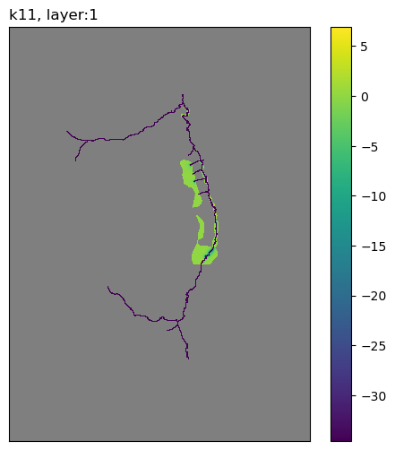
The composite group contains sensitivities of the performance measure to the model inputs, summed across all adjoint solutions.
[18]:
grp = hdf["composite"]
plot_keys = [
    i
    for i in grp.keys()
    if len(grp[i].shape) == 3 and ("k11" in i or "wel" in i or "ss" in i)
]
plot_keys
[18]:
['k11', 'ss', 'wel6_q']
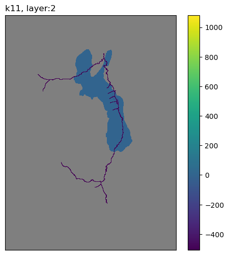
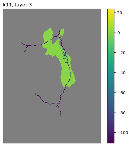
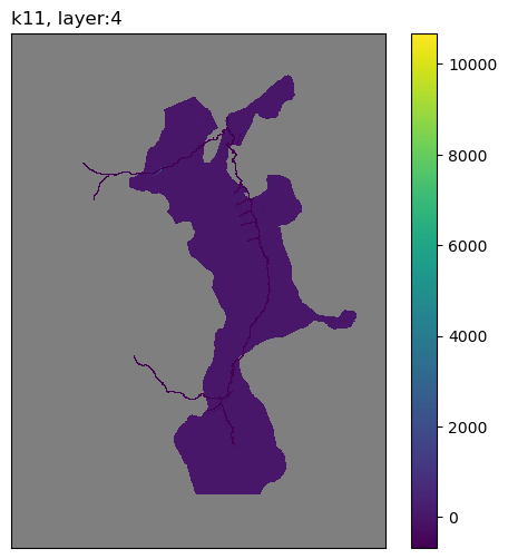
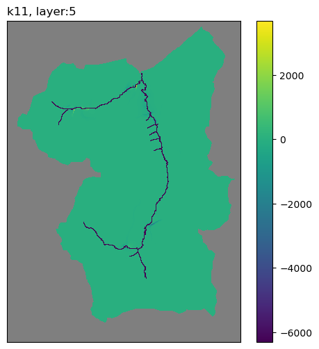
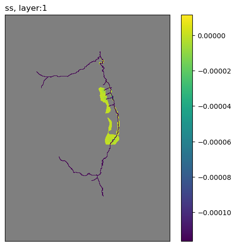
Here is a simple routine to plot these sensitivities.
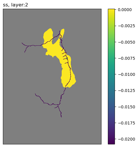
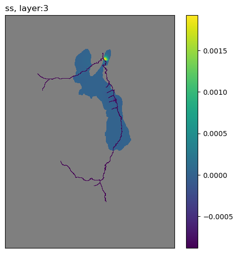
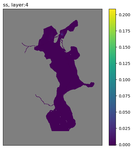
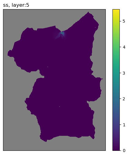
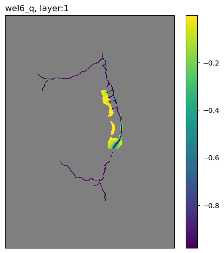
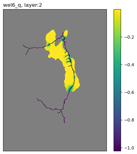
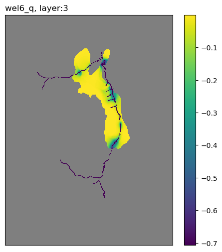
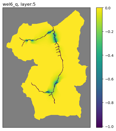
[19]:
for pkey in plot_keys:
    arr = grp[pkey][:]
    for k, karr in enumerate(arr):
        karr[karr == 0.0] = np.nan
        fig, ax = plot_model(k, karr)
        ax.set_title(pkey + f", layer:{k + 1}", loc="left")
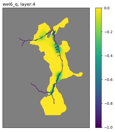
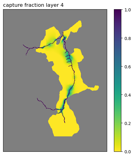
One especially well-known plot in this context is the so-called capture fraction map:
[20]:
arr = grp["wel6_q"][3, :, :]
arr[arr == 0.0] = np.nan
fig, ax = plot_model(3, np.abs(arr), cmap="viridis_r")
ax.set_title("capture fraction layer 4", loc="left");
[21]:
arr = grp["wel6_q"][4, :, :]
arr[arr == 0.0] = np.nan
fig, ax = plot_model(4, np.abs(arr), cmap="viridis_r")
ax.set_title("capture fraction layer 5", loc="left");
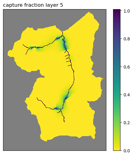
This plot shows capture fraction: the proportion of groundwater captured from the simulated surface-water/groundwater flux if a groundwater well were added in a given model cell. Traditionally, this would be calculated by adding a well or other specified-flux boundary in each model cell, rerunning the model, recording how the surface water/groundwater flux changed, and normalizing that change by the applied rate for every active cell. That can take a long time. With the adjoint approach, the so-called adjoint state for this performance measure is simply the negative of the capture fraction: it shows how the simulated gw-sw flux changes in response to a unit injection of water in each active model cell.